
Background

Hospitality industry is growing, with more and more people spending their money for vacation and leisure activities. People may only lodge into a hotel when it’s a holiday season or a special event, thus the demand for staying room is not equally distributed accross the year. To maximize the revenue gained by the hotel, the management often employed a pricing strategy, one of them being raising the room rate when the demand is high and making a promo when the demand is low. Thus, the ability to accurately forecast the future demand is very important and became a vital part on the pricing scheme. The demand for different segment of customer may differ and forecasting become harder as it may requires different model for different segment.
This post will focus on fitting and tuning different forecasting models using purrr package on a real dataset .
Library and Setup
Below is the list of required packages if you wish to reproduce the results. The full source code for this post is available at my github repository .
# Data Wrangling
library(tidyverse)
library(lubridate)

# Visualization
library(ggthemes)
library(scales)

# Time Series
library(forecast)
library(tseries)
library(padr)

# Machine Learning
library(rsample)
library(recipes)
Hotel Demand Forecasting
Import Data
Let’s import the dataset. The data is acquired from Nuno et al. (2019) . The data consists of around 119,390 booking transactions from 2 hotel: an anonymous city hotel from Lisbon and a resort hotel from Algarve. The dataset comprehend bookings due to arrive between the 1st of July of 2015 and the 31st of August 2017, including bookings that effectively arrived and bookings that were canceled. There is so much to explore from this data, but we will only focus on demand forecasting.

hotel <- read.csv("data_input/hotel_bookings.csv")

head(hotel, 10)
#> hotel is_canceled lead_time arrival_date_year arrival_date_month
#> 1 Resort Hotel 0 342 2015 July
#> 2 Resort Hotel 0 737 2015 July
#> 3 Resort Hotel 0 7 2015 July
#> 4 Resort Hotel 0 13 2015 July
#> 5 Resort Hotel 0 14 2015 July
#> 6 Resort Hotel 0 14 2015 July
#> 7 Resort Hotel 0 0 2015 July
#> 8 Resort Hotel 0 9 2015 July
#> 9 Resort Hotel 1 85 2015 July
#> 10 Resort Hotel 1 75 2015 July
#> arrival_date_week_number arrival_date_day_of_month stays_in_weekend_nights
#> 1 27 1 0
#> 2 27 1 0
#> 3 27 1 0
#> 4 27 1 0
#> 5 27 1 0
#> 6 27 1 0
#> 7 27 1 0
#> 8 27 1 0
#> 9 27 1 0
#> 10 27 1 0
#> stays_in_week_nights adults children babies meal country market_segment
#> 1 0 2 0 0 BB PRT Direct
#> 2 0 2 0 0 BB PRT Direct
#> 3 1 1 0 0 BB GBR Direct
#> 4 1 1 0 0 BB GBR Corporate
#> 5 2 2 0 0 BB GBR Online TA
#> 6 2 2 0 0 BB GBR Online TA
#> 7 2 2 0 0 BB PRT Direct
#> 8 2 2 0 0 FB PRT Direct
#> 9 3 2 0 0 BB PRT Online TA
#> 10 3 2 0 0 HB PRT Offline TA/TO
#> distribution_channel is_repeated_guest previous_cancellations
#> 1 Direct 0 0
#> 2 Direct 0 0
#> 3 Direct 0 0
#> 4 Corporate 0 0
#> 5 TA/TO 0 0
#> 6 TA/TO 0 0
#> 7 Direct 0 0
#> 8 Direct 0 0
#> 9 TA/TO 0 0
#> 10 TA/TO 0 0
#> previous_bookings_not_canceled reserved_room_type assigned_room_type
#> 1 0 C C
#> 2 0 C C
#> 3 0 A C
#> 4 0 A A
#> 5 0 A A
#> 6 0 A A
#> 7 0 C C
#> 8 0 C C
#> 9 0 A A
#> 10 0 D D
#> booking_changes deposit_type agent company days_in_waiting_list
#> 1 3 No Deposit NULL NULL 0
#> 2 4 No Deposit NULL NULL 0
#> 3 0 No Deposit NULL NULL 0
#> 4 0 No Deposit 304 NULL 0
#> 5 0 No Deposit 240 NULL 0
#> 6 0 No Deposit 240 NULL 0
#> 7 0 No Deposit NULL NULL 0
#> 8 0 No Deposit 303 NULL 0
#> 9 0 No Deposit 240 NULL 0
#> 10 0 No Deposit 15 NULL 0
#> customer_type adr required_car_parking_spaces total_of_special_requests
#> 1 Transient 0.0 0 0
#> 2 Transient 0.0 0 0
#> 3 Transient 75.0 0 0
#> 4 Transient 75.0 0 0
#> 5 Transient 98.0 0 1
#> 6 Transient 98.0 0 1
#> 7 Transient 107.0 0 0
#> 8 Transient 103.0 0 1
#> 9 Transient 82.0 0 1
#> 10 Transient 105.5 0 0
#> reservation_status reservation_status_date
#> 1 Check-Out 2015-07-01
#> 2 Check-Out 2015-07-01
#> 3 Check-Out 2015-07-02
#> 4 Check-Out 2015-07-02
#> 5 Check-Out 2015-07-03
#> 6 Check-Out 2015-07-03
#> 7 Check-Out 2015-07-03
#> 8 Check-Out 2015-07-03
#> 9 Canceled 2015-05-06
#> 10 Canceled 2015-04-22Data Description:
hotel : Hotel (Resort Hotel or City Hotel)
is_canceled : Value indicating if the booking was canceled (1) or not (0)
lead_time : Number of days that elapsed between the entering date of the booking into the PMS and the arrival date
arrival_date_year : Year of arrival date
arrival_date_month : Month of arrival date
arrival_date_week_number : Week number of year for arrival date
arrival_date_day_of_month : Day of arrival date
stays_in_weekend_nights : Number of weekend nights (Saturday or Sunday) the guest stayed or booked to stay at the hotel
stays_in_week_nights : Number of week nights (Monday to Friday) the guest stayed or booked to stay at the hotel
adults : Number of adults
children : Number of children
babies : Number of babies
meal : Type of meal booked. Categories are presented in standard hospitality meal packages:
- Undefined/SC – no meal package
- BB – Bed & Breakfast
- HB – Half board (breakfast and one other meal – usually dinner)
- FB – Full board (breakfast, lunch and dinner)
country : Country of origin. Categories are represented in the ISO 3155–3:2013 format
market_segment : Market segment designation. In categories, the term “TA” means “Travel Agents” and “TO” means “Tour Operators”
distribution_channel : Booking distribution channel. The term “TA” means “Travel Agents” and “TO” means “Tour Operators”
is_repeated_guest : Value indicating if the booking name was from a repeated guest (1) or not (0)
previous_cancellations : Number of previous bookings that were cancelled by the customer prior to the current booking
previous_bookings_not_canceled : Number of previous bookings not cancelled by the customer prior to the current booking
reserved_room_type : Code of room type reserved. Code is presented instead of designation for anonymity reasons.
assigned_room_type : Code for the type of room assigned to the booking. Sometimes the assigned room type differs from the reserved room type due to hotel operation reasons (e.g. overbooking) or by customer request. Code is presented instead of designation for anonymity reasons.
booking_changes : Number of changes/amendments made to the booking from the moment the booking was entered on the PMS until the moment of check-in or cancellation
deposit_type : Indication on if the customer made a deposit to guarantee the booking. This variable can assume three categories:
- No Deposit – no deposit was made
- Non Refund * a deposit was made in the value of the total stay cost
- Refundable – a deposit was made with a value under the total cost of stay.
agent : ID of the travel agency that made the booking
company : ID of the company/entity that made the booking or responsible for paying the booking. ID is presented instead of designation for anonymity reasons
days_in_waiting_list : Number of days the booking was in the waiting list before it was confirmed to the customer
customer_type : Type of booking, assuming one of four categories:
- Contract - when the booking has an allotment or other type of contract associated to it
- Group – when the booking is associated to a group
- Transient – when the booking is not part of a group or contract, and is not associated to other transient booking
- Transient-party – when the booking is transient, but is associated to at least other transient booking
adr : Average Daily Rate as defined by dividing the sum of all lodging transactions by the total number of staying nights
required_car_parking_spaces : Number of car parking spaces required by the customer
total_of_special_requests : Number of special requests made by the customer (e.g. twin bed or high floor)
reservation_status : Reservation last status, assuming one of three categories:
- Canceled – booking was canceled by the customer
- Check-Out – customer has checked in but already departed
- No-Show – customer did not check-in and did inform the hotel of the reason why
reservation_status_date : Date at which the last status was set. This variable can be used in conjunction with the ReservationStatus to understand when was the booking canceled or when did the customer checked-out of the hotel
Data Preprocessing
Before we analyze the data, you may notice that the date is scattered in separate columns. We will unite them together to get a proper arrival date column.
hotel <- hotel %>%
  unite("arrival_date", arrival_date_year, arrival_date_month, arrival_date_day_of_month, sep = "-") %>%
  mutate(arrival_date = ymd(arrival_date))

head(hotel)
#> hotel is_canceled lead_time arrival_date arrival_date_week_number
#> 1 Resort Hotel 0 342 2015-07-01 27
#> 2 Resort Hotel 0 737 2015-07-01 27
#> 3 Resort Hotel 0 7 2015-07-01 27
#> 4 Resort Hotel 0 13 2015-07-01 27
#> 5 Resort Hotel 0 14 2015-07-01 27
#> 6 Resort Hotel 0 14 2015-07-01 27
#> stays_in_weekend_nights stays_in_week_nights adults children babies meal
#> 1 0 0 2 0 0 BB
#> 2 0 0 2 0 0 BB
#> 3 0 1 1 0 0 BB
#> 4 0 1 1 0 0 BB
#> 5 0 2 2 0 0 BB
#> 6 0 2 2 0 0 BB
#> country market_segment distribution_channel is_repeated_guest
#> 1 PRT Direct Direct 0
#> 2 PRT Direct Direct 0
#> 3 GBR Direct Direct 0
#> 4 GBR Corporate Corporate 0
#> 5 GBR Online TA TA/TO 0
#> 6 GBR Online TA TA/TO 0
#> previous_cancellations previous_bookings_not_canceled reserved_room_type
#> 1 0 0 C
#> 2 0 0 C
#> 3 0 0 A
#> 4 0 0 A
#> 5 0 0 A
#> 6 0 0 A
#> assigned_room_type booking_changes deposit_type agent company
#> 1 C 3 No Deposit NULL NULL
#> 2 C 4 No Deposit NULL NULL
#> 3 C 0 No Deposit NULL NULL
#> 4 A 0 No Deposit 304 NULL
#> 5 A 0 No Deposit 240 NULL
#> 6 A 0 No Deposit 240 NULL
#> days_in_waiting_list customer_type adr required_car_parking_spaces
#> 1 0 Transient 0 0
#> 2 0 Transient 0 0
#> 3 0 Transient 75 0
#> 4 0 Transient 75 0
#> 5 0 Transient 98 0
#> 6 0 Transient 98 0
#> total_of_special_requests reservation_status reservation_status_date
#> 1 0 Check-Out 2015-07-01
#> 2 0 Check-Out 2015-07-01
#> 3 0 Check-Out 2015-07-02
#> 4 0 Check-Out 2015-07-02
#> 5 1 Check-Out 2015-07-03
#> 6 1 Check-Out 2015-07-03Exploratory Data Analysis
Market Segments
For each hotel, we have several market segments as mentioned earlier in the data description. In order to maximize our revenue, we will forecast the most profitable market segment. First, we will look at the number of transactions for each market segment on each hotel.
hotel %>%
  count(hotel, market_segment, is_canceled) %>%
  group_by(hotel) %>%
  mutate(total = sum(n),
         ratio = n/total,
         is_canceled = ifelse(is_canceled == 0, "No", "Yes")) %>%
  ungroup() %>%
  mutate(market_segment = tidytext::reorder_within(market_segment, ratio, hotel)) %>%
  ggplot(aes(ratio, market_segment, fill = is_canceled)) +
  geom_col(position = "dodge") +
  labs(x = "Percentage", y = "Market Segment",
       title = "Hotel Demand by Market Segment",
       fill = "Booking Canceled") +
  facet_wrap(~hotel, scales = "free_y") +
  scale_x_continuous(labels = percent_format(accuracy = 1)) +
  scale_fill_manual(values = c("skyblue", "firebrick")) +
  tidytext::scale_y_reordered() +
  theme_pander() +
  theme(legend.position = "top")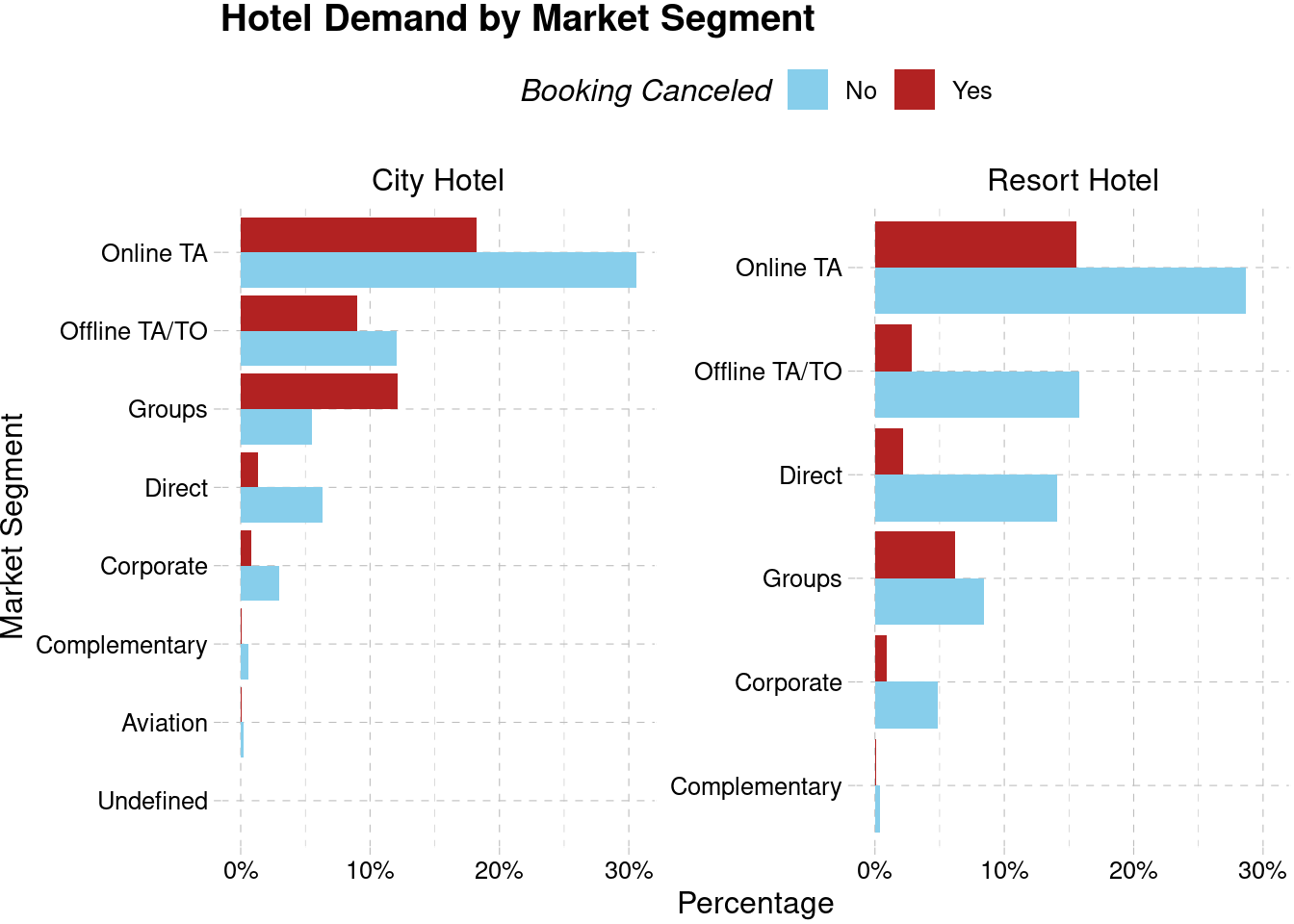
Based on the result, most of the booking done via travel agent, either online or offline, which combined together contributes more than 40% of the non-canceled total transactions. The other segment don’t have much transactions, but perhaps we would like to see the revenue generated by each market segment by looking at the Average Daily Rate (ADR). Average Daily Rate as defined by dividing the sum of all lodging transactions by the total number of staying nights. Therefore, the higher ADR means more revenue generated for each staying night.
hotel %>%
  filter(is_canceled == F) %>%
  group_by(hotel, market_segment) %>%
  summarise(adr = sum(adr)) %>%
  mutate(total = sum(adr),
         ratio = adr/total) %>%
  ungroup() %>%
  mutate(market_segment = tidytext::reorder_within(market_segment, ratio, hotel)) %>%
  ggplot(aes(ratio, market_segment)) +
  geom_col(fill = "firebrick") +
  facet_wrap(~hotel, scales = "free_y") +
  tidytext::scale_y_reordered() +
  scale_x_continuous(labels = percent_format(accuracy = 1)) +
  theme_pander() +
  labs(x = NULL, y = NULL,
       title = "ADR Contributions by Market Segments")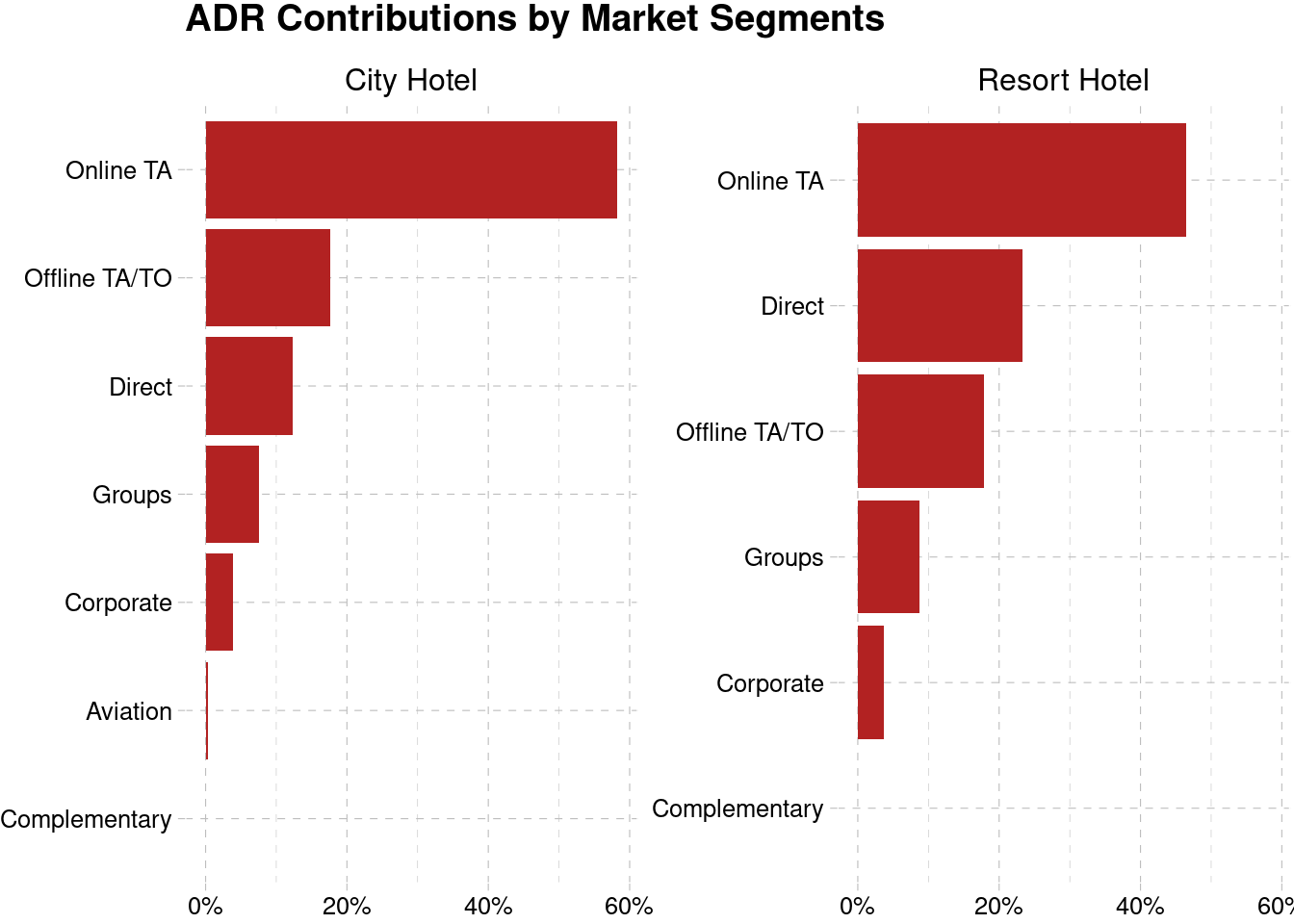
Total ADR generated from online travel agent is the highest both in the city hotel and the resort hotel. The segment of offline travel agent and direct has a little margin with each other, with direct segment has the higher contribution in resort hotel even though it has lower number of transactions. This give us the top 3 market segments, both in term of quantity and profitability. We will focus on this segments for the rest of the analysis.
Time Series Analysis
We want to forecast the demand of lodging for both city hotel and resort hotel. Based on the previous exploration, we will use only the data from segment online travel agent, offline travel agent and direct. We will consider both canceled and non-canceled transactions to reflect the demand.
hotel_city <- hotel %>%
  filter(hotel == "City Hotel",
         market_segment %>% str_detect("TA|Direct"))

hotel_resort <- hotel %>%
  filter(hotel == "Resort Hotel",
         market_segment %>% str_detect("TA|Direct"))

hotel_agg_city <- hotel_city %>%
  group_by(arrival_date) %>%
  summarise(demand = n())

hotel_agg_resort <- hotel_resort %>%
  group_by(arrival_date) %>%
  summarise(demand = n())

head(hotel_agg_city, 10)
#> # A tibble: 10 × 2
#> arrival_date demand
#> <date> <int>
#> 1 2015-07-01 79
#> 2 2015-07-02 8
#> 3 2015-07-03 3
#> 4 2015-07-04 6
#> 5 2015-07-05 8
#> 6 2015-07-06 10
#> 7 2015-07-07 18
#> 8 2015-07-08 8
#> 9 2015-07-09 6
#> 10 2015-07-10 7Let’s look at the series of demand for each hotel.
hotel_agg_city   %>%
  mutate(hotel = "City Hotel") %>%
  bind_rows(hotel_agg_resort %>% mutate(hotel = "Resort Hotel")) %>%
  ggplot(aes(arrival_date, demand)) +
  geom_line(color = "dodgerblue4") +
  theme_pander() +
  facet_wrap(~hotel, ncol = 1) +
  labs(x = NULL, y = "Demand", title = "Hotel Booking Demand")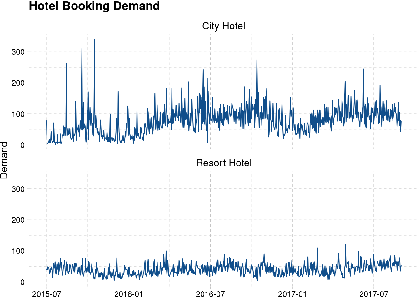
The demand for city hotel has a higher fluctuation compared to the resort hotel. This may be caused by several factors, including the room capacity, since we don’t know the room capacity for each hotel. There are also some spikes in demand for city hotel during the late 2015. We will inspect further by dividing the series by market segment. We will also need to make the series have constant interval of time, which is a daily interval in our case.
# summarizing data
hotel_agg_city <- hotel_city %>%
  group_by(arrival_date, market_segment) %>%
  summarise(demand = n())

hotel_agg_resort <- hotel_resort %>%
  group_by(arrival_date, market_segment) %>%
  summarise(demand = n())

# join city hotel and resort hotel
hotel_agg <- hotel_agg_city %>%
  mutate(hotel = "City Hotel") %>%
  bind_rows(hotel_agg_resort %>% mutate(hotel = "Resort Hotel")) %>%
  ungroup()

# padding
start_interval <-  ymd(range(hotel$arrival_date)[1])
end_interval <- ymd(range(hotel$arrival_date)[2])

hotel_pad <- hotel_agg %>%
  group_by(hotel, market_segment) %>%
  pad(start_val = start_interval, end_val = end_interval) %>%
  replace_na(list(demand = 0)) %>%
  ungroup()

hotel_pad %>%
  ggplot(aes(arrival_date, demand, color = market_segment)) +
  geom_line() +
  theme_pander() +
  theme(legend.position = "top") +
  facet_wrap(~hotel, ncol = 1, scales = "free_y") +
  labs(x = NULL, y = "Demand", title = "Hotel Demand", color = NULL) +
  scale_color_manual(values = c("firebrick", "skyblue", "orange"))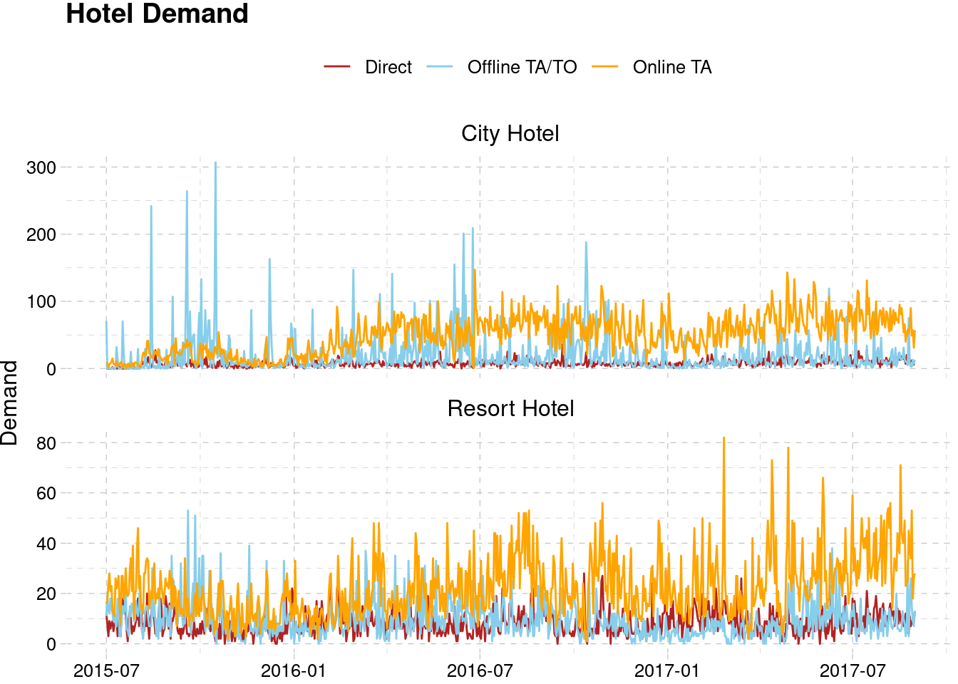
The behaviour for each segment is quite different, so we will forecast them separately. At this point, we will have 6 different time series to be forecasted for 3 different segments on each hotel.
Seasonality Analysis
Before we proceed to create a forecasting model. We will try to gain more insight regarding the customer behaviour by looking at the seasonality of the demand. Since we have too many series, we will only explore the most lucrative market segment, that is the segment of online TA. We will look at the behaviour for both the city hotel and the resort hotel.
Weekly Seasonality
First, we will look at the weekly seasonality. The weekly seasonality will help us to understand when does people more frequently do check in? Our common sense will tell us that perhaps weekend should be the one where people start to check in. However, weekly seasonality may have a weak strength since people are not regularly go to vacation or rent a hotel.
The following figures is the weekly seasonality of the online TA segment for the city hotel. It has a negative seasonality on the weekend (Saturday and Sunday) and has a high positive seasonality in Tuesday. Thus, the hotel is more likely to have less visitor on the weekend, perhaps because the hotel is not designed to be a vacation hotel and more of a business or transit hotel.
city_weekly <- hotel_agg_city %>%
  filter(market_segment == "Online TA") %>%
  ts(frequency = 7) %>%
  decompose()

city_weekly$seasonal %>%
  matrix(ncol = 7, byrow = T) %>%
  t() %>%
  as.data.frame() %>%
  select(V1) %>%
  mutate(day = wday(head(hotel_agg_city %>% filter(market_segment == "Online TA") %>% pull(arrival_date) , 7), label = T)) %>%
  ggplot(aes(day, V1, fill = V1)) +
  geom_col(show.legend = F) +
  geom_hline(yintercept = 0 ) +
  labs(x = NULL, y = "seasonality", title = "Weekly Seasonality of City Hotel, Online TA Segment ") +
  scale_fill_gradient2(low = "firebrick4", mid = "skyblue", high = "dodgerblue4") +
  theme_pander()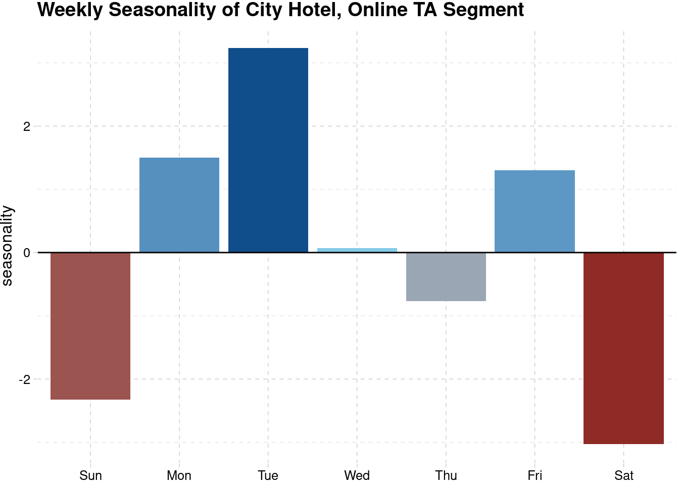
Next, we will look at the weekly seasonality of the Online TA segment of the Resort Hotel as well.
resort_weekly <- hotel_agg_resort %>%
  filter(market_segment == "Online TA") %>%
  ts(frequency = 7) %>%
  decompose()

resort_weekly$seasonal %>%
  matrix(ncol = 7, byrow = T) %>%
  t() %>%
  as.data.frame() %>%
  select(V1) %>%
  mutate(day = wday(head(hotel_agg_resort %>% filter(market_segment == "Online TA") %>% pull(arrival_date) , 7), label = T)) %>%
  ggplot(aes(day, V1, fill = V1)) +
  geom_col(show.legend = F) +
  geom_hline(yintercept = 0 ) +
  labs(x = NULL, y = "seasonality", title = "Weekly Seasonality of Resort Hotel, Online TA Segment ") +
  scale_fill_gradient2(low = "firebrick4", mid = "skyblue", high = "dodgerblue4") +
  theme_pander()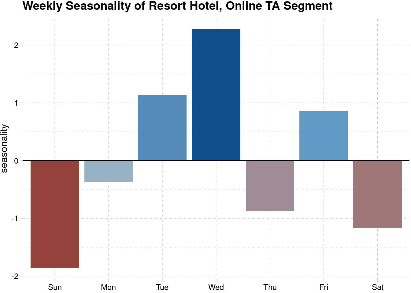
The customer behaviour is quite the same, with strong positive seasonality happened during Wednesday and negative seasonality during Sunday. It is natural that the number of arrival is dropping during Sunday, since people will go back to their and home do the ordinary activities on Monday. Another reason is perhaps because Monday is the day that most of the monuments/museusms etc are closed in Portugal so if people checked in on Sunday evening the don’t have much to visit during the next day. The peak seasonality in Wednesday may signal that people want to spent more time for the upcoming weekend or people just want to avoid the crowd during weekend.
Monthly Seasonality
We will also check the monthly seasonality and see at what month does it reach its highest and lowest point. The first one is the city hotel.
city_monthly <- hotel_agg_city %>%
  filter(market_segment == "Online TA") %>%
  mutate(date = floor_date(arrival_date, "month")) %>%
  group_by(date) %>%
  summarise(demand = sum(demand)) %>%
  ungroup()

monthly_ts <- ts(city_monthly,frequency = 12) %>%
  decompose()

monthly_ts$seasonal %>%
  matrix(ncol = 12, byrow = T) %>%
  t() %>%
  as.data.frame() %>%
  select(V1) %>%
  mutate(month = month(head(city_monthly$date, 12), label = T)) %>%
  ggplot(aes(month, V1, fill = V1)) +
  geom_col(show.legend = F) +
  geom_hline(yintercept = 0 ) +
  labs(x = NULL, y = "seasonality", title = "Monthly Seasonality of City Hotel, Online TA Segment ") +
  scale_fill_gradient2(low = "firebrick4", mid = "skyblue", high = "dodgerblue4") +
  theme_pander()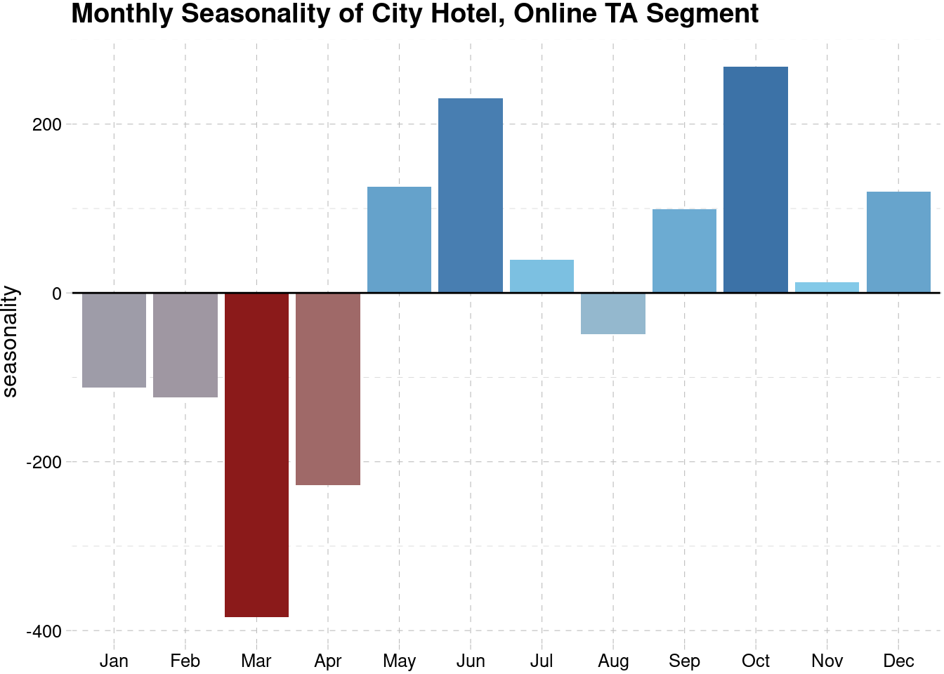
The next one is the online TA segment in Resort Hotel. The seasonality reach its highest point during October and same with the city hotel, it reach the lowest point on March.
resort_monthly <- hotel_agg_resort %>%
  filter(market_segment == "Online TA") %>%
  mutate(date = floor_date(arrival_date, "month")) %>%
  group_by(date) %>%
  summarise(demand = sum(demand)) %>%
  ungroup()

monthly_ts <- ts(resort_monthly,frequency = 12) %>%
  decompose()

monthly_ts$seasonal %>%
  matrix(ncol = 12, byrow = T) %>%
  t() %>%
  as.data.frame() %>%
  select(V1) %>%
  mutate(month = month(head(resort_monthly$date, 12), label = T)) %>%
  ggplot(aes(month, V1, fill = V1)) +
  geom_col(show.legend = F) +
  geom_hline(yintercept = 0 ) +
  labs(x = NULL, y = "seasonality", title = "Monthly Seasonality of resort Hotel, Online TA Segment ") +
  scale_fill_gradient2(low = "firebrick4", mid = "skyblue", high = "dodgerblue4") +
  theme_pander()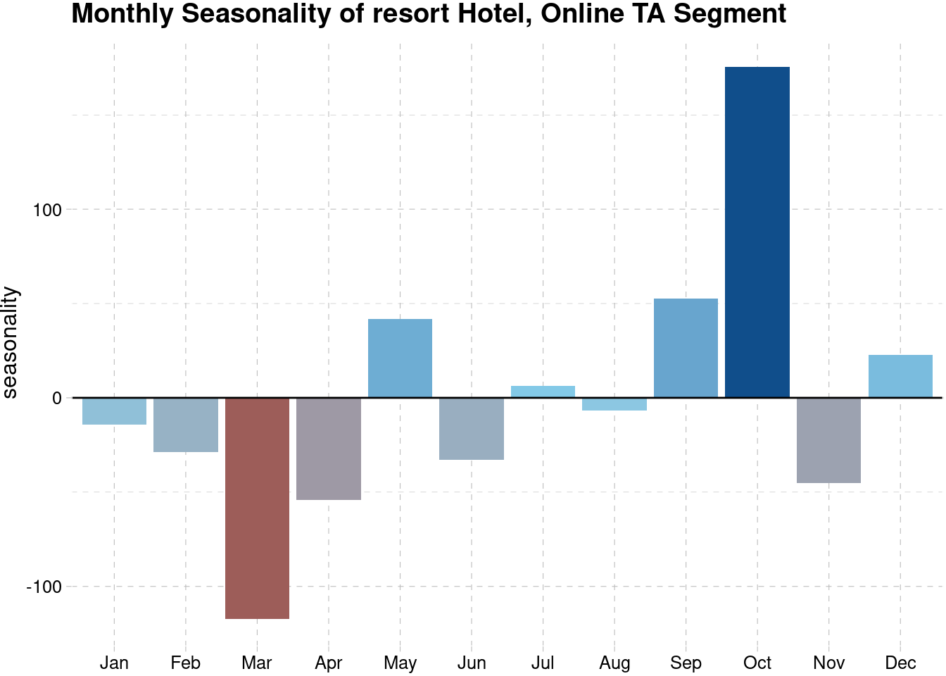
Based on both graphs, the high and positive seasonality happens around May-June and September-October. The highest negative seasonality happens in March. Both Lisbon and Algarve are located in Portugal. According to Audley Travels , the best time to visit Portugal is in spring (March-May), when the country is in bloom and waking after the winter. You could also go in fall (between September and October) when the sun is still shining, the weather is warm, and many of the crowds have dispersed. However, the negative seasonality in March and April perhaps tell us that the weather is still too cold to travel around and people love to spend more time to go for vacation during September and October. The summer holiday of school, which is span from late June to early September, have a good influence toward the city hotel seasonality.

September and October are two of the best months to visit Portugal. The weather is still warm and pleasant, and the temperatures are much more manageable for sightseeing or hiking. It’s also a wonderful time to visit many of Portugal’s wineries with the grape harvest in full swing. The beaches are also much quieter.
For the next sections, we will focus on the forecasting of the demand using various machine learning methods.
Cross-Validation
We will split the data into training dataset and testing dataset, with testing dataset consists of the last 30 days from the full dataset.
# get total number of observations
n_data <- hotel %>%
  count(arrival_date) %>%
  nrow()

# data train
hotel_train <- hotel_pad %>%
  group_by(hotel, market_segment) %>%
  slice( 1:(n_data-30) )

# data test
hotel_test <- hotel_pad %>%
  group_by(hotel, market_segment) %>%
  slice( -(n_data-30:n_data) )

tail(hotel_train, 10)
#> # A tibble: 10 × 4
#> # Groups: hotel, market_segment [1]
#> arrival_date market_segment demand hotel
#> <date> <chr> <dbl> <chr>
#> 1 2017-07-23 Online TA 26 Resort Hotel
#> 2 2017-07-24 Online TA 46 Resort Hotel
#> 3 2017-07-25 Online TA 25 Resort Hotel
#> 4 2017-07-26 Online TA 32 Resort Hotel
#> 5 2017-07-27 Online TA 33 Resort Hotel
#> 6 2017-07-28 Online TA 36 Resort Hotel
#> 7 2017-07-29 Online TA 51 Resort Hotel
#> 8 2017-07-30 Online TA 23 Resort Hotel
#> 9 2017-07-31 Online TA 44 Resort Hotel
#> 10 2017-08-01 Online TA 49 Resort HotelForecasting Methods
We will do forecasting for each segment of each hotel. This is done to capture the pattern of each series since they have different characteristics and doing an aggregated forecast may result in higher error. Thus, we will have 6 different series, 3 for each hotel. Since we have 6 series to forecast, manually fitting and tuning the model will be tedious and take a long time. We will use purrr to efficiently fitting and evaluating the model in order to get the best model for each series based on the Mean Absolute Error (MAE) and Root Mean Squared Error (RMSE) values. MAE is chosen due to it’s interpretability while RMSE is chosen because it is sensitive to large errors. We don’t use Mean Absolute Percentage Error because it did not perform really well when the actual data has or close to zero value, despite being easier to interpret.
\[MAE = \frac{\Sigma_{i = 1}^{n} (y_i- \hat{y_i})}{n}\]
\[RMSE = \sqrt\frac{\Sigma_{i = 1}^{n} (y_i-\hat{y_i} )^2}{n}\]
Before we proceed, we will do forecasting method for the aggregated time series by combining all demand into a single series. This will function as a benchmark for the subsequent forecasting.
train_agg <- hotel_train %>%
  group_by(arrival_date) %>%
  summarise(demand = sum(demand))

test_agg <- hotel_test %>%
  group_by(arrival_date) %>%
  summarise(demand = sum(demand))

head(train_agg, 10)
#> # A tibble: 10 × 2
#> arrival_date demand
#> <date> <dbl>
#> 1 2015-07-01 118
#> 2 2015-07-02 52
#> 3 2015-07-03 43
#> 4 2015-07-04 55
#> 5 2015-07-05 53
#> 6 2015-07-06 55
#> 7 2015-07-07 53
#> 8 2015-07-08 34
#> 9 2015-07-09 38
#> 10 2015-07-10 49With a weekly seasonality and using ARIMA method, here is the result of the forecast on the next 30 days. The forecast give us MAE of 21, which mean that the model will have different around 21 demands compared to the actual testing dataset in average and RMSE around 26.
train_ts <- ts(train_agg$demand, frequency = 7)

arima_agg <- auto.arima(train_ts)

forecast_agg <- forecast(arima_agg, h = 30)

accuracy(forecast_agg, test_agg$demand) %>%
  as.data.frame()
#> ME RMSE MAE MPE MAPE MASE
#> Training set 0.4580128 37.73934 28.13519 -10.16052 27.86560 0.7628458
#> Test set -8.0150470 26.31801 21.25028 -8.68376 15.88266 0.5761712
#> ACF1
#> Training set 0.00200618
#> Test set NAWe will see if by separating the series will give us better forecast performance.
First, we will nest the dataset, making our data into a list of 6 separate time series.
# nesting data train
train_list <- hotel_train %>%
  select(-arrival_date) %>%
  unite("series", hotel, market_segment, sep = "_") %>%
  nest(-series)

# nesting data test
test_list <- hotel_test %>%
  select(-arrival_date) %>%
  unite("series", hotel, market_segment, sep = "_") %>%
  nest(-series)

head(train_list)
#> # A tibble: 6 × 2
#> series data
#> <chr> <list>
#> 1 City Hotel_Direct <tibble [763 × 1]>
#> 2 City Hotel_Offline TA/TO <tibble [763 × 1]>
#> 3 City Hotel_Online TA <tibble [763 × 1]>
#> 4 Resort Hotel_Direct <tibble [763 × 1]>
#> 5 Resort Hotel_Offline TA/TO <tibble [763 × 1]>
#> 6 Resort Hotel_Online TA <tibble [763 × 1]>The column data consists of a list of the demand for each series. For example, the following is the series for the City Hotel with Direct Segment.
train_list$data[[1]] %>%
  head()
#> # A tibble: 6 × 1
#> demand
#> <dbl>
#> 1 0
#> 2 0
#> 3 0
#> 4 0
#> 5 0
#> 6 0Preprocessing Specification
We will try several preprocess approach since there is a possibility that transformed data are performing better than the original scale. We will use the following treatment:
- No data transformation
- Squared value
- Scaled value, data will be normalized using z-score
- Log transformation
recipe_spec <- list(
  normal_spec = function(x) x, # no transformation
  squared_spec = function(x) sqrt(x), # square the demand value
  scale_spec = function(x) scale(x), # normalize the demand value with Z-score
  log_spec = function(x) log(x+1) # convert demand to log
) %>%
  enframe(name = "preprocess_name", value = "preprocess_spec")

recipe_spec
#> # A tibble: 4 × 2
#> preprocess_name preprocess_spec
#> <chr> <list>
#> 1 normal_spec <fn>
#> 2 squared_spec <fn>
#> 3 scale_spec <fn>
#> 4 log_spec <fn>We also need to create a function to reverse the scaled to value into the original value for later model evaluation. For example, if the data is being square rooted, then we need to scale it back by squaring the data.
# reverse function to scale back for model evaluation
reverse_spec <- list(

  normal_spec = function(x, y) {
    y <- y
    return(x)
    },

  squared_spec = function(x, y) {
    y <- y
    return(x^2)
    },

  scale_spec = function(x, y) x * sd(y) + mean(y),

  log_spec = function(x,y) {
    y <- y
    return(exp(x)-1)
  }
) %>%
  enframe(name = "reverse_name", value = "reverse_spec")

# joint the preprocess and the scale-back function
recipe_spec <- recipe_spec %>%
  bind_cols(reverse_spec)
Seasonality Specification
The next step is to specify the seasonal period for the series. We will try several seasonal period, including:
- weekly seasonality
- monthly seasonality
- annual seasonality
- weekly and monthly seasonality (multi-seasonal)
- weekly and annual seasonality (multi-seasonal)
seasonal_forecast <- list(
  weekly = function(x) ts(x, frequency = 7),
  monthly = function(x) ts(x, frequency = 7*4),
  weekly_monthly = function(x) msts(x, seasonal.periods = c(7, 7*4)),
  weekly_annual = function(x) msts(x, seasonal.periods = c(7, 365)),
  annual = function(x) ts(x, frequency = 365)
  ) %>%
  enframe(name = "season_name", value = "season_spec")
Impute Outlier
We will also try to preprocess the data by whether an outlier should be replaced or not. If the outlier is replaced, we will identify the outlier and estimate the replacement using the tsoutliers function. Residuals are identified by fitting a loess curve for non-seasonal data and via a periodic STL decomposition for seasonal data.
outlier_spec <- list(
  normal_spec = function(x) x, # no transformation

  out_spec = function(x){
    outlier_place <- tsoutliers(x)
    x[outlier_place$index] <- outlier_place$replacement
    return(x)
  }
) %>%
  enframe(name = "outlier_name", value = "out_spec")
Model Specification
Next, we will specify the model the data will be fit into. The model includes:
- ARIMA
- STL + ETS model
- STL + ARIMA
method_forecast <- list(
  arima  = function(x) auto.arima(x),
  stl_ets = function(x) stlm(x, method = "ets"),
  stl_arima = function(x) stlm(x, method = "arima")
  ) %>%
  enframe(name = "model_name", value = "model_spec")
Model Fitting
Below is the combination for each specification on each series. For 6 different series, we will have 5 different seasonality specification, 3 different models and other specifications. Therefore, we will 540 different combinations. We will choose the best model based on the RMSE and MAE value on the testing dataset. For example, the first row is the time series for City Hotel with Direct Segment. This data will be transformed using log (log_spec) with annual seasonality and fitted with time series model using ARIMA.
# combine the data with the specification
train_crossing <- crossing(train_list, recipe_spec, seasonal_forecast, outlier_spec, method_forecast )

test_crossing <- crossing(test_list, recipe_spec, seasonal_forecast, outlier_spec, method_forecast)

train_crossing %>%
  head()
#> # A tibble: 6 × 12
#> series data preprocess_name preprocess_spec reverse_name reverse_spec
#> <chr> <list> <chr> <list> <chr> <list>
#> 1 City Hote… <tibble … log_spec <fn> log_spec <fn>
#> 2 City Hote… <tibble … log_spec <fn> log_spec <fn>
#> 3 City Hote… <tibble … log_spec <fn> log_spec <fn>
#> 4 City Hote… <tibble … log_spec <fn> log_spec <fn>
#> 5 City Hote… <tibble … log_spec <fn> log_spec <fn>
#> 6 City Hote… <tibble … log_spec <fn> log_spec <fn>
#> # … with 6 more variables: season_name <chr>, season_spec <list>,
#> # outlier_name <chr>, out_spec <list>, model_name <chr>, model_spec <list>The following code produce the transformation process for the data before fitted into model.
# model fitting and evaluation
transformed_data <- map2(.x = train_crossing$data,
                         .y = train_crossing$preprocess_spec,
                         .f = ~exec( .y, .x)
                         )
The following code do all process from transforming data into time series, fitting them into the model and forecast demands for the next 30 days.
# fitting and forecasting
forecast_map <- transformed_data %>%

  # Convert data to time series with different seasonalities
  map2(.y = train_crossing$season_spec,
       .f = ~exec(.y, .x)) %>%

  # Transform outlier
  map2(.y = train_crossing$out_spec,
       .f = ~exec(.y, .x)) %>%

  # Fit data to time series model
  map2(.y = train_crossing$model_spec,
       .f =  ~exec(.y,.x)) %>%

  # Forecast for the next 30 days
  map(forecast, h = 30) %>%

  # Take the mean of the forecast
  map(~pluck(.x, "mean")) %>%

  map(as.numeric)
Forecasting Result
Below is the result for our modeling process for the first time series.
# Result of the first time series
forecast_map[[1]]
#> [1] 2.346707 2.338587 2.338587 2.338587 2.338587 2.338587 2.338587 2.338587
#> [9] 2.338587 2.338587 2.338587 2.338587 2.338587 2.338587 2.338587 2.338587
#> [17] 2.338587 2.338587 2.338587 2.338587 2.338587 2.338587 2.338587 2.338587
#> [25] 2.338587 2.338587 2.338587 2.338587 2.338587 2.338587We use MAE and RMSE to measures and compares the performance of each model.
# scale-back the data to original scale value
forecast_trans <- list()

for (i in 1:length(forecast_map)) {
  forecast_trans[[i]] <- train_crossing$reverse_spec[[i]]( x = forecast_map[[i]], y = transformed_data[[i]])
}

forecast_trans[[1]]
#> [1] 9.451100 9.366579 9.366579 9.366579 9.366579 9.366579 9.366579 9.366579
#> [9] 9.366579 9.366579 9.366579 9.366579 9.366579 9.366579 9.366579 9.366579
#> [17] 9.366579 9.366579 9.366579 9.366579 9.366579 9.366579 9.366579 9.366579
#> [25] 9.366579 9.366579 9.366579 9.366579 9.366579 9.366579# calculate MAE
mae_list <- forecast_trans %>%
map2(.y = test_crossing$data,
.f = ~yardstick::mae_vec(.x %>% as.numeric(), .y$demand))
rmse_list <- forecast_trans %>%
map2(.y = test_crossing$data,
.f = ~yardstick::rmse_vec(.x %>% as.numeric(), .y$demand))
# show result
train_crossing %>%
separate(series, c("hotel", "market_segment"), sep = "_") %>%
select_if(is.character) %>%
bind_cols(mae = mae_list %>% as.numeric()) %>%
bind_cols(rmse = rmse_list %>% as.numeric()) %>%
select(hotel, market_segment, mae, rmse, everything()) %>%
head(10)#> # A tibble: 10 × 9
#> hotel market_segment mae rmse preprocess_name reverse_name season_name
#> <chr> <chr> <dbl> <dbl> <chr> <chr> <chr>
#> 1 City Hot… Direct 3.79 4.63 log_spec log_spec annual
#> 2 City Hot… Direct 11.7 13.9 log_spec log_spec annual
#> 3 City Hot… Direct 10.6 12.8 log_spec log_spec annual
#> 4 City Hot… Direct 3.79 4.63 log_spec log_spec annual
#> 5 City Hot… Direct 11.7 13.9 log_spec log_spec annual
#> 6 City Hot… Direct 10.6 12.8 log_spec log_spec annual
#> 7 City Hot… Direct 3.79 4.63 log_spec log_spec monthly
#> 8 City Hot… Direct 3.85 4.71 log_spec log_spec monthly
#> 9 City Hot… Direct 3.79 4.64 log_spec log_spec monthly
#> 10 City Hot… Direct 3.79 4.63 log_spec log_spec monthly
#> # … with 2 more variables: outlier_name <chr>, model_name <chr>Below is the best configuration for each series based on the lowest RMSE, since RMSE give more penality towards large error. To interpret the MAE values, we need to consider the range of the data, shown as the standar deviation of the data.
# best configuration for each series
best_adjust <- train_crossing %>%
  separate(series, c("hotel", "market_segment"), sep = "_") %>%
  bind_cols(mae = mae_list %>% as.numeric()) %>%
  bind_cols(rmse = rmse_list %>% as.numeric()) %>%
  group_by(hotel, market_segment) %>%
  arrange(rmse) %>%
  slice(1)

# show the result
metric_crossing <- train_list %>% crossing(list(mean = mean, std_dev = sd) %>% enframe(name = "type", value = "metric"))

metric_crossing %>%
  bind_cols(value = map2(.x = metric_crossing$data,
                         .y = metric_crossing$metric,
                         .f = ~exec(.y, unlist(.x))) %>% unlist()
            ) %>%
  select(series, type, value) %>%
  pivot_wider(names_from = type, values_from = value) %>%
  separate(series, c("hotel", "market_segment"), sep = "_") %>%
  left_join(best_adjust) %>%
  select_if(~is.list(.) == F) %>%
  select(-reverse_name) %>%
  select(hotel, market_segment, mae, rmse,  mean, std_dev, everything()) %>%
  arrange(rmse)
#> # A tibble: 6 × 10
#> hotel market_segment mae rmse mean std_dev preprocess_name season_name
#> <chr> <chr> <dbl> <dbl> <dbl> <dbl> <chr> <chr>
#> 1 Resort H… Direct 2.21 2.65 8.14 4.85 normal_spec weekly
#> 2 City Hot… Direct 3.43 4.17 7.53 4.83 normal_spec weekly
#> 3 Resort H… Offline TA/TO 4.26 6.09 9.39 7.38 log_spec weekly_ann…
#> 4 Resort H… Online TA 8.71 11.0 21.8 11.7 squared_spec weekly
#> 5 City Hot… Offline TA/TO 8.80 13.7 21.4 32.0 normal_spec weekly
#> 6 City Hot… Online TA 13.2 16.2 48.1 28.5 squared_spec weekly
#> # … with 2 more variables: outlier_name <chr>, model_name <chr>Since we don’t have much data, only two years of transactions, the model performance may not perform so well. However, judging from the MAE value, the performance is quite acceptable, with most of the error values are less than the value of one standard deviation. Compared to the aggregated data on the first forecast which have MAE of 21, we have lower MAE value for each series, which give us an evidence that by making a separate forecasting models for each market segment will make the model more accurate.
# Aggregated time series performance
accuracy(forecast_agg, test_agg$demand) %>%
  as.data.frame() %>%
  slice(2) %>%
  select(MAE, RMSE)
#> MAE RMSE
#> Test set 21.25028 26.31801Below is the forecasting result for each series. The red line indicate the actual demand value while the blue line indicate the forecast value. The blue area represent area with 80% prediction interval while the light blue are represent the 95% prediction interval. Most of the actual demand is still inside the forecasting intervals.
Resort Hotel, Online TA
model_best <- map2(.x = best_adjust$data,
                   .y = best_adjust$season_spec,
                   .f =  ~exec(.y,.x)) %>%
  map2(.y = best_adjust$model_spec,
       .f =  ~exec(.y,.x)
       )

data_test <- test_list$data[[6]] %>%
  msts(start = 110, seasonal.periods =  7)

model_best[[6]] %>%
  forecast(h = 30 ) %>%
  autoplot() +
  autolayer(data_test, series = "Data Test") +
  scale_color_manual(values = "firebrick") +
  labs(subtitle = "Resort Hotel, Online TA",
       y = "Demand", x  = NULL) +
  theme_pander() +
  scale_x_continuous(limits = c(100, 115) ,
                     labels = as.Date.numeric(seq(100,115,5)*7-7, origin = range(hotel$arrival_date)[1])) +
  theme(legend.position = "top")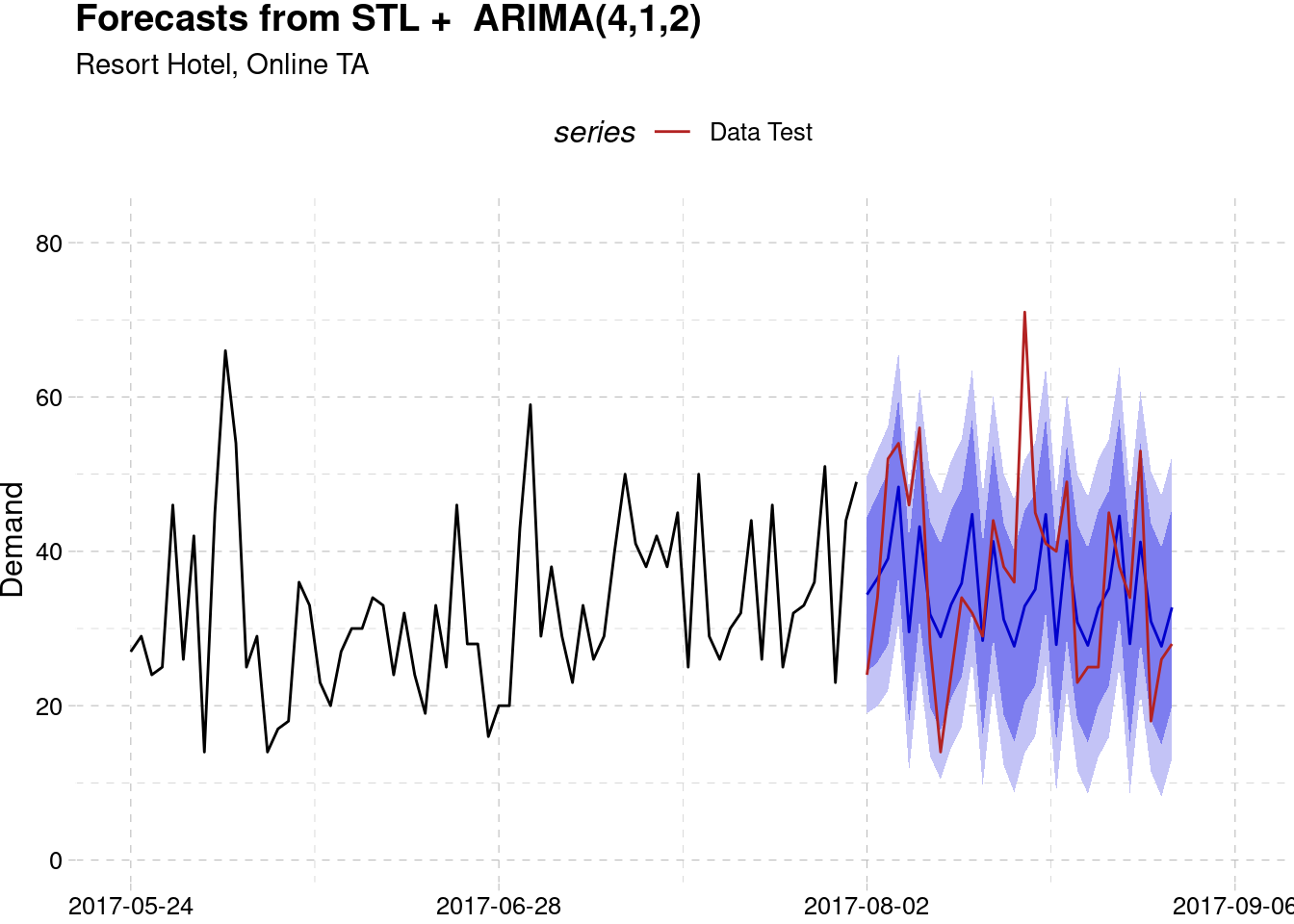
model_best[[6]]$residuals %>%
  as.data.frame() %>%
  ggplot(aes(x)) +
  geom_density(fill = "skyblue", alpha = 0.7, color = "white") +
  labs(x = "Residuals", y = "Density",
       title = "Residuals Distribution") +
  theme_pander()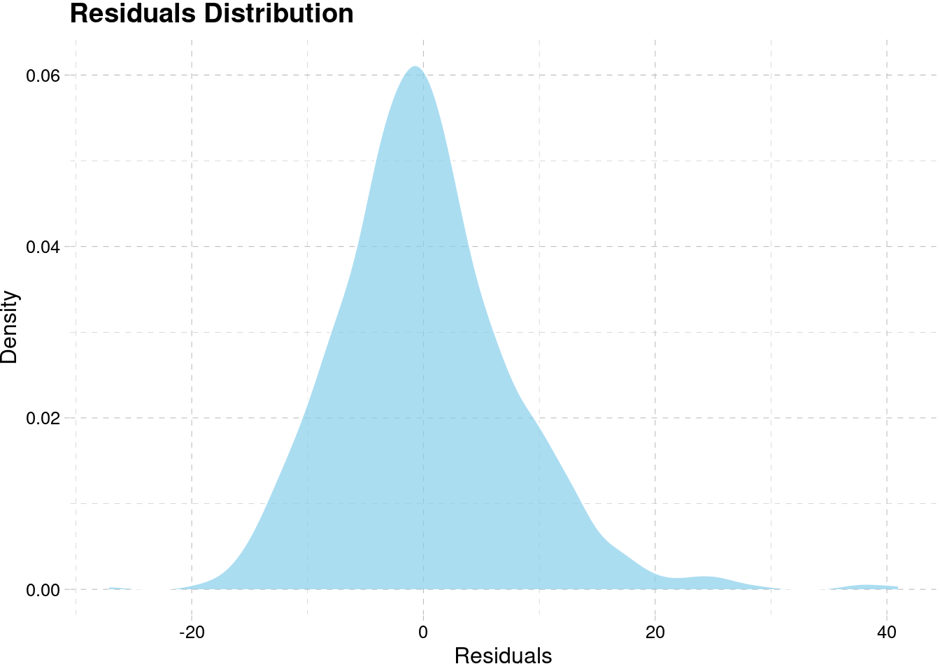
City Hotel, Online TA
data_test <- test_list$data[[3]] %>%
  ts(start = 110, frequency = 7)

model_best[[3]] %>%
  forecast(h = 30 ) %>%
  autoplot() +
  autolayer(data_test, series = "Data Test") +
  scale_color_manual(values = "firebrick") +
  labs(subtitle = "City Hotel, Online TA",
       y = "Demand", x  = NULL) +
  theme_pander() +
  scale_x_continuous(limits = c(100, 115),
                     labels = as.Date.numeric(seq(100,115,5)*7-7, origin = range(hotel$arrival_date)[1])) +
  theme(legend.position = "top")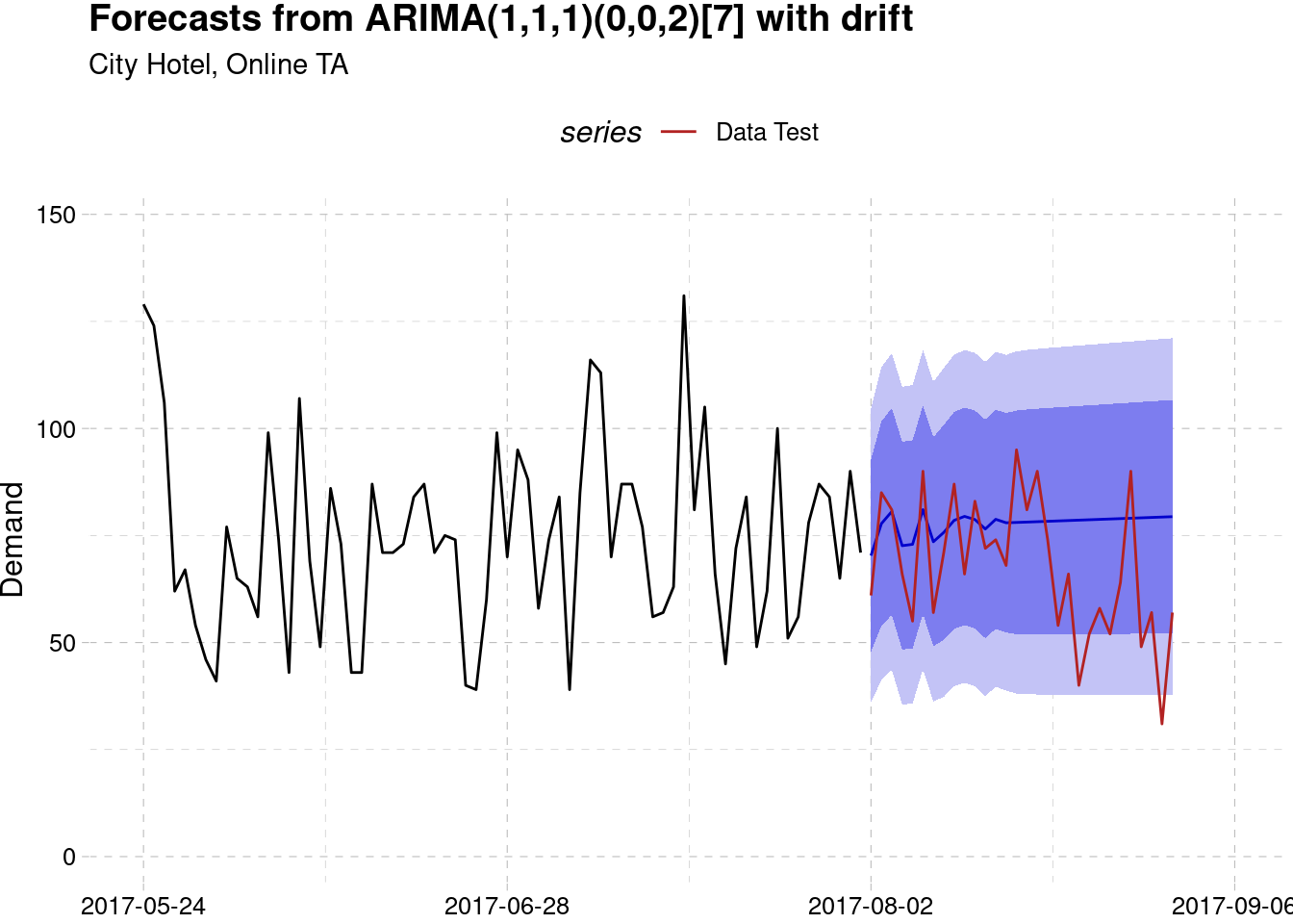
model_best[[3]]$residuals %>%
  as.data.frame() %>%
  ggplot(aes(x)) +
  geom_density(fill = "skyblue", alpha = 0.7, color = "white") +
  labs(x = "Residuals", y = "Density",
       title = "Residuals Distribution") +
  theme_pander()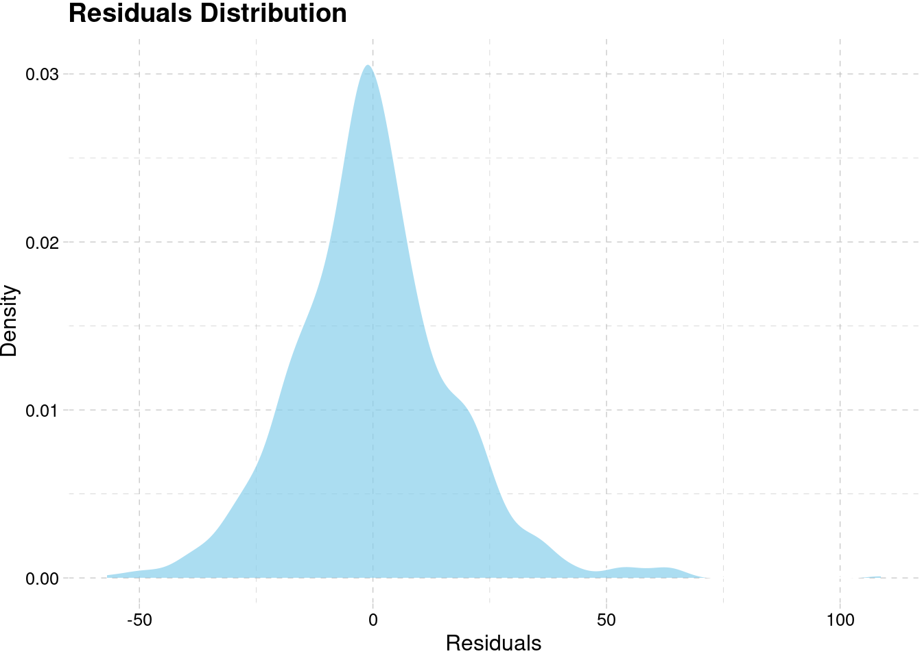
Resort Hotel, Offline TA/TO
data_test <- test_list$data[[5]] %>% msts(start = 3.090411, seasonal.periods = c(7, 365))

model_best[[5]] %>%
  forecast(h = 30 ) %>%
  autoplot() +
  autolayer(data_test, series = "Data Test") +
  scale_color_manual(values = "firebrick") +
  labs(subtitle = "Resort Hotel, Offline TA/TO",
       y = "Demand", x  = NULL) +
  theme_pander() +
  scale_x_continuous(limits = c(3, 3.2),
                     labels = as.Date.numeric(seq(3,3.2,0.05)*365-365, origin = range(hotel$arrival_date)[1])) +
  theme(legend.position = "top")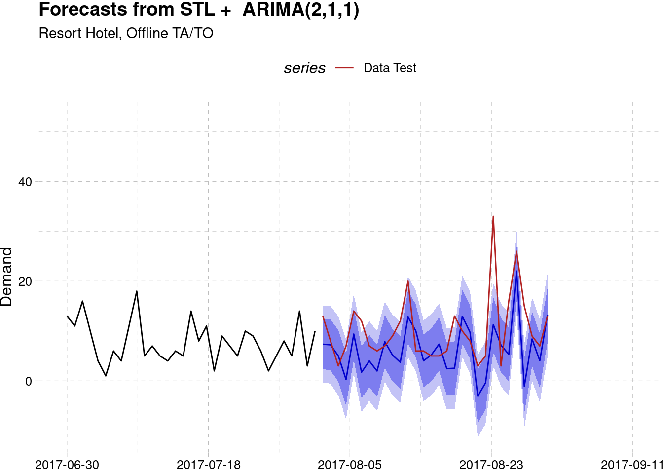
model_best[[5]]$residuals %>%
  as.data.frame() %>%
  ggplot(aes(x)) +
  geom_density(fill = "skyblue", alpha = 0.7, color = "white") +
  labs(x = "Residuals", y = "Density",
       title = "Residuals Distribution") +
  theme_pander()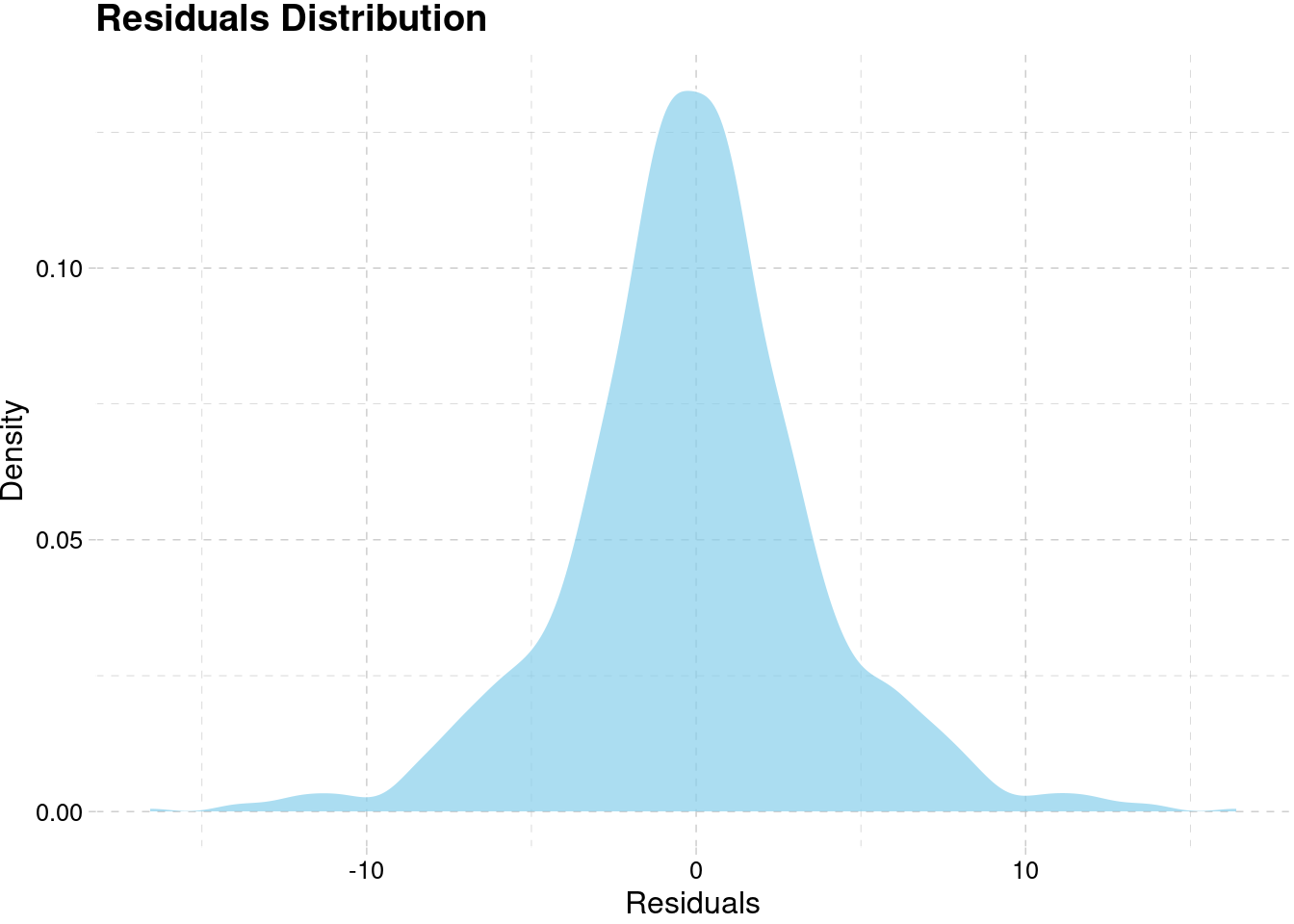
City Hotel, Offline TA/TO
data_test <- test_list$data[[2]] %>% ts(start = 110, frequency = 7)

model_best[[2]] %>%
  forecast(h = 30 ) %>%
  autoplot() +
  autolayer(data_test, series = "Data Test") +
  scale_color_manual(values = "firebrick") +
  labs(subtitle = "City Hotel, Offline TA/TO",
       y = "Demand", x  = NULL) +
  theme_pander() +
  scale_x_continuous(limits = c(100, 115),
                     labels = as.Date.numeric(seq(100,115,5)*7-7, origin = range(hotel$arrival_date)[1])) +
  theme(legend.position = "top")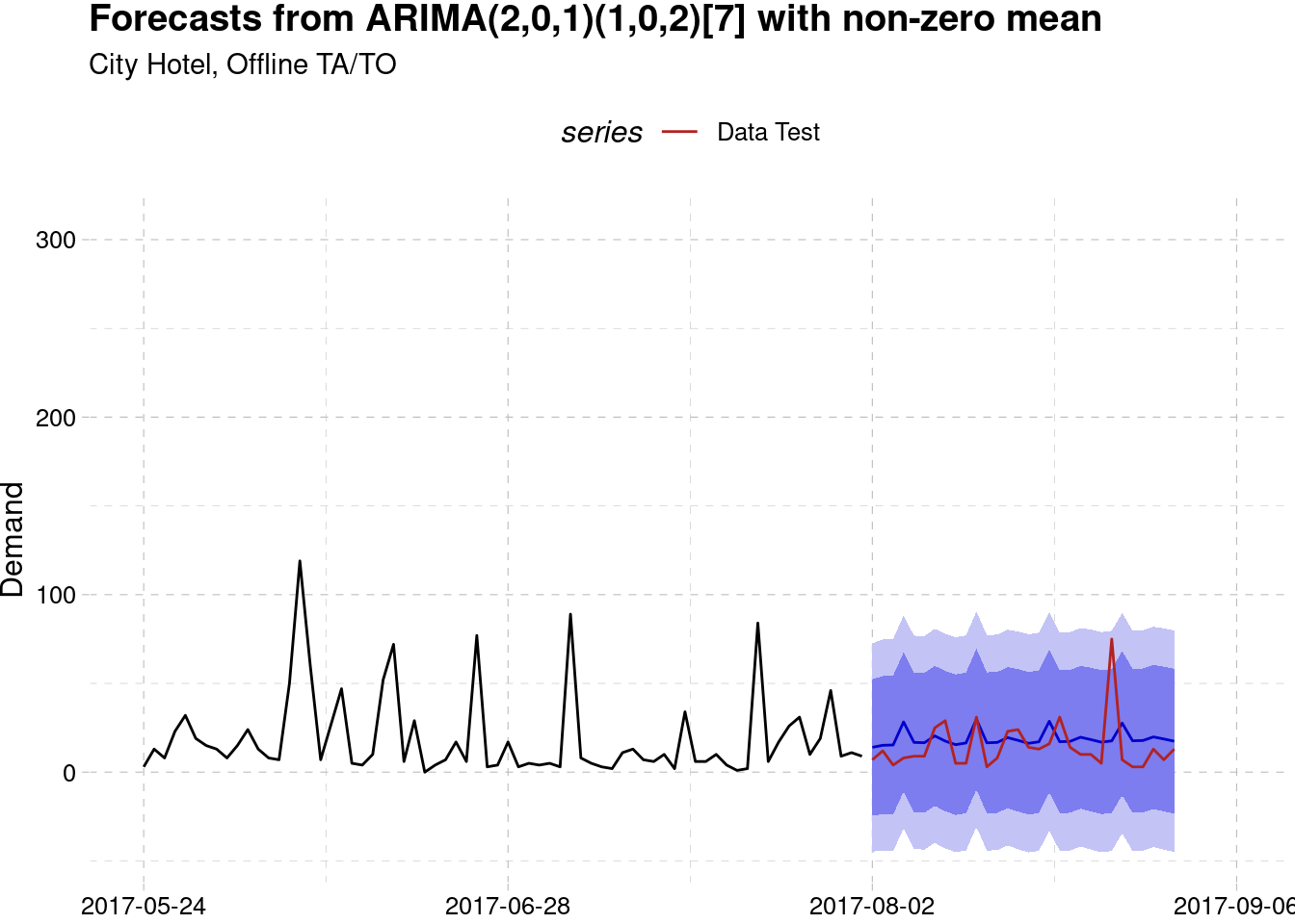
model_best[[2]]$residuals %>%
  as.data.frame() %>%
  ggplot(aes(x)) +
  geom_density(fill = "skyblue", alpha = 0.7, color = "white") +
  labs(x = "Residuals", y = "Density",
       title = "Residuals Distribution") +
  theme_pander()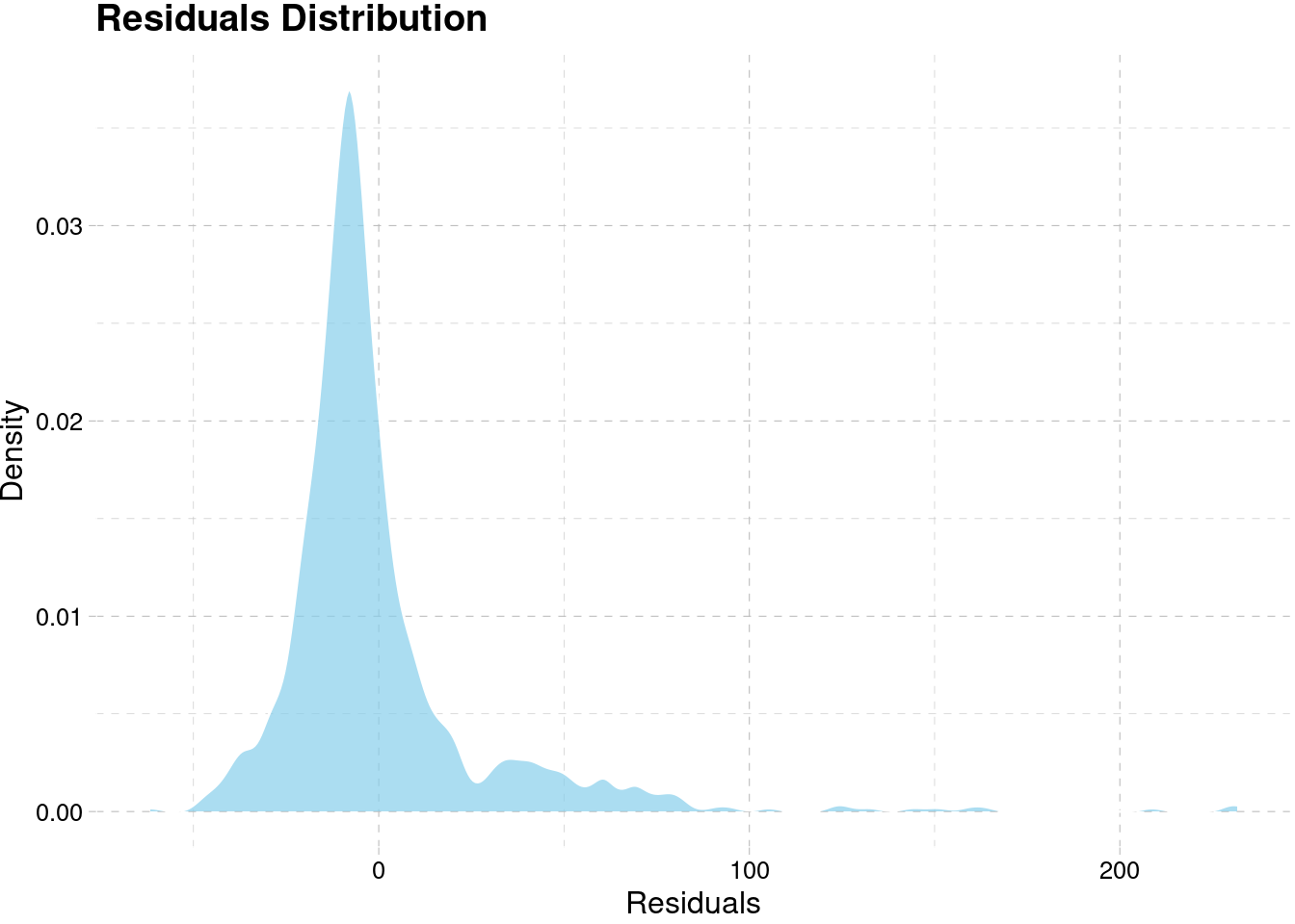
Resort Hotel, Direct
data_test <- test_list$data[[4]] %>% ts(start = 110, frequency = 7)

model_best[[4]] %>%
  forecast(h = 30 ) %>%
  autoplot() +
  autolayer(data_test, series = "Data Test") +
  scale_color_manual(values = "firebrick") +
  labs(subtitle = "Resort Hotel, Direct",
       y = "Demand", x  = NULL) +
  theme_pander() +
  scale_x_continuous(limits = c(100, 115),
                     labels = as.Date.numeric(seq(100,115,5)*7-7, origin = range(hotel$arrival_date)[1])) +
  theme(legend.position = "top")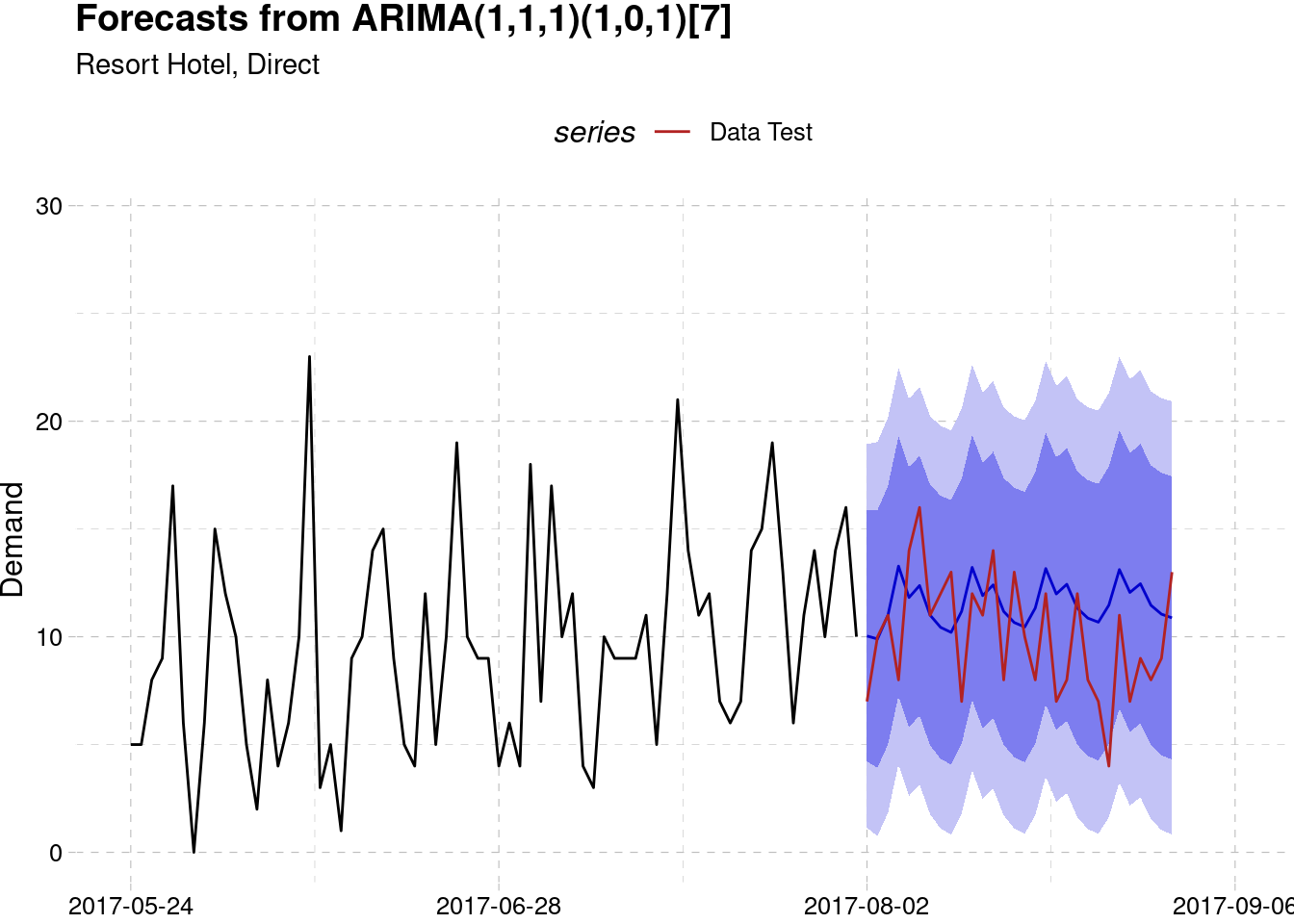
model_best[[4]]$residuals %>%
  as.data.frame() %>%
  ggplot(aes(x)) +
  geom_density(fill = "skyblue", alpha = 0.7, color = "white") +
  labs(x = "Residuals", y = "Density",
       title = "Residuals Distribution") +
  theme_pander()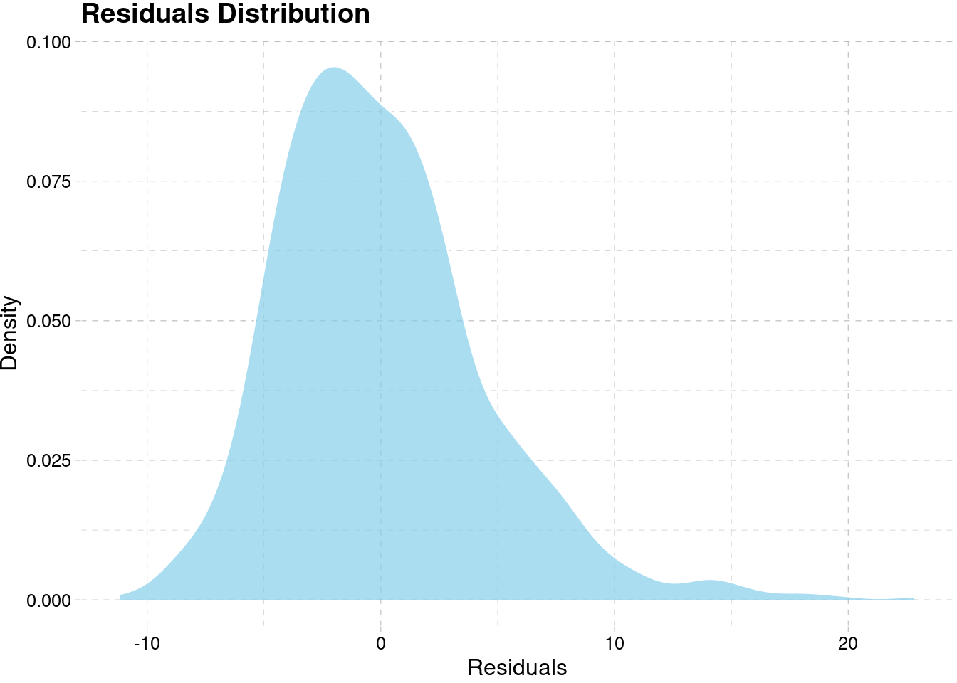
City Hotel, Direct
data_test <- test_list$data[[1]] %>% ts(start = 110, frequency = 7)

model_best[[1]] %>%
  forecast(h = 30 ) %>%
  autoplot() +
  autolayer(data_test, series = "Data Test") +
  scale_color_manual(values = "firebrick") +
  labs(subtitle = "City Hotel, Direct",
       y = "Demand", x  = NULL) +
  theme_pander() +
  scale_x_continuous(limits = c(100, 115),
                     labels = as.Date.numeric(seq(100,115,5)*7-7, origin = range(hotel$arrival_date)[1])) +
  theme(legend.position = "top")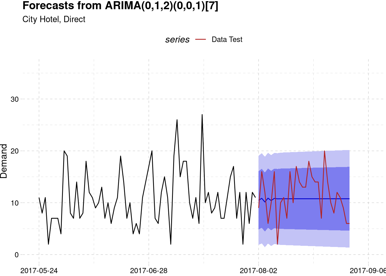
model_best[[1]]$residuals %>%
  as.data.frame() %>%
  ggplot(aes(x)) +
  geom_density(fill = "skyblue", alpha = 0.7, color = "white") +
  labs(x = "Residuals", y = "Density",
       title = "Residuals Distribution") +
  theme_pander()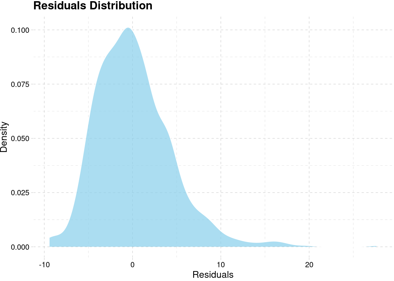
Model Assumption Checking
Autocorrelation
The autocorrelation can be checked using the Ljung-Box test. If there are correlations between residuals, then there is information left in the residuals which should be used in computing forecasts.
best_adjust %>%
  select(hotel, market_segment) %>%
  bind_cols(
      map(model_best, ~Box.test(.x$residuals, type = "Lj")) %>%
  unlist() %>%
  matrix(ncol = 5, byrow = T) %>%
  as.data.frame() %>%
  select(4:3) %>%
  rename(p_value = V3, test = V4) %>%
  mutate(p_value = p_value %>%
           as.character() %>%
           as.numeric() %>%
           round(4))
  )
#> # A tibble: 6 × 4
#> # Groups: hotel, market_segment [6]
#> hotel market_segment test p_value
#> <chr> <chr> <chr> <dbl>
#> 1 City Hotel Direct Box-Ljung test 0.976
#> 2 City Hotel Offline TA/TO Box-Ljung test 0.971
#> 3 City Hotel Online TA Box-Ljung test 0.769
#> 4 Resort Hotel Direct Box-Ljung test 0.854
#> 5 Resort Hotel Offline TA/TO Box-Ljung test 0.959
#> 6 Resort Hotel Online TA Box-Ljung test 0.959The results suggests that all of our models don’t have any autocorrelation based on the non-significant p-value.
Normality
We will also check if the residuals for each model is normally distributed using Shapiro-Wilk Test. If the residuals are not normally distributed, it will lead to a biased parameter and less optimal forecast. This is also indicate that we can still tweak our model to get a better performance.
best_adjust %>%
  select(hotel, market_segment) %>%
  bind_cols(
    mean_error = map(model_best, ~mean(.$residuals)) %>%
      as.numeric() %>%
      round(5)
  ) %>%
  bind_cols(
    median_error = map(model_best, ~median(.$residuals)) %>%
      as.numeric() %>%
      round(5)
  ) %>%
  bind_cols(
      map(model_best, ~shapiro.test(.x$residuals)) %>%
        unlist() %>%
        matrix(ncol = 4, byrow = T) %>%
        as.data.frame() %>%
        select(3:2) %>%
        rename(p_value = V2, test = V3)
  ) %>%
  rename(segment = market_segment) %>%
  mutate(p_value = p_value %>%
           as.character() %>%
           as.numeric() %>%
           number(accuracy = 0.00001))
#> # A tibble: 6 × 6
#> # Groups: hotel, segment [6]
#> hotel segment mean_error median_error test p_value
#> <chr> <chr> <dbl> <dbl> <chr> <chr>
#> 1 City Hotel Direct 0.180 -0.387 Shapiro-Wilk normali… 0.00000
#> 2 City Hotel Offline TA/… 0.104 -6.74 Shapiro-Wilk normali… 0.00000
#> 3 City Hotel Online TA 0.0146 -0.898 Shapiro-Wilk normali… 0.00000
#> 4 Resort Hot… Direct 0.0442 -0.586 Shapiro-Wilk normali… 0.00000
#> 5 Resort Hot… Offline TA/… -0.0813 -0.142 Shapiro-Wilk normali… 0.00000
#> 6 Resort Hot… Online TA 0.211 -0.426 Shapiro-Wilk normali… 0.00000Based on the result, all of our model didn’t fulfill the normality assumption for the residuals. The positive mean of error signify that the model is underestimate the forecast while negative mean error means the model is overestimate. If we look at the median of error, all of our models are underestimate on the training set. They might be influenced by the presence of an outlier value such as a really high demand especially on the early part of the series. This suggest that we can improve the model further in order to get better performance.
Conclusion
This article has illustrated how R and functional programming of purrr can help us to do flexible forecasting for multiple time series models. We have tried to do hotel demand forecasting using a real-world datasets with two years worth of data. We also have tried to analyze the series pattern for each hotel and segment and fit the best model for each one of them with a satisfying results. The next step perhaps is to enhance the model further either by using another time series model, incorporate predictor by the unused variables from the original dataset or transforming the data.
 More details
 More details
Share this post
Twitter
Facebook
LinkedIn