Introduction

One of many things to consider when we want to choose a machine learning model is the interpretability: can we analyze what variables or certain values that contribute toward particular class or target? Some models can be easily interpreted, such as the linear or logistic regression model and decision trees, but interpreting more complex model such as random forest and neural network can be challenging. This sometimes drive the data scientist to choose more interpretable model since they need to communicate it to their manager or higher rank, who perhaps are not familiar with machine learning. The downside is, in general, interpretable model has lower performance in term of accuracy or precision, making them less useful and potentially dangerous for production. Therefore, there is a growing need on how to interpret a complex and black box model easily.

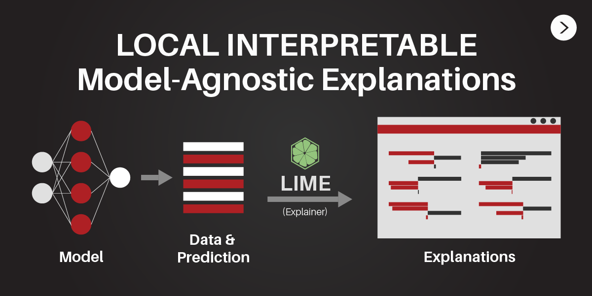
There exist a method called LIME, a novel explanation technique that explains the predictions of any classifier in an interpretable and faithful manner, by learning an interpretable model locally around the prediction. Here we will see how LIME works on binary classification problem of employee attrition. By understanding on how our model works, we can have more advantage and could act wiser on what should we do.

Local Interpretable Model-Agnostic Explanations (LIME)

LIME characteristics

Let’s understand some of the LIME characteristic (Ribeiro et al., 2016):

• Interpretable

Provide qualitative understanding between the input variables and the response. Interpretability must take into account the user’s limitations. Thus, a linear model, a gradient vector or an additive model may or may not be interpretable. For example, if hundreds or thousands of features significantly contribute to a prediction, it is not reasonable to expect any user to comprehend why the prediction was made, even if individual weights can be inspected. This requirement further implies that explanations should be easy to understand, which is not necessarily true of the features used by the model, and thus the “input variables” in the explanations may need to be different than the features. Finally, the notion of interpretability also depends on the target audience. Machine learning practitioners may be able to interpret small Bayesian networks, but laymen may be more comfortable with a small number of weighted features as an explanation.

• Local Fidelity

Although it is often impossible for an explanation to be completely faithful unless it is the complete description of the model itself, for an explanation to be meaningful it must at least be locally faithful, i.e. it must correspond to how the model behaves in the vicinity of the instance being predicted. We note that local fidelity does not imply global fidelity: features that are globally important may not be important in the local context, and vice versa. While global fidelity would imply local fidelity, identifying globally faithful explanations that are interpretable remains a challenge for complex models.

• Model-Agnostic

An explainer should be able to explain any model, and thus be model-agnostic (i.e. treat the original model as a black box). Apart from the fact that many state of the art classifiers are not currently interpretable, this also provides flexibility to explain future classifiers.

How LIME works

The generalized algorithm LIME applies is (Boehmke, 2018):

(1) Given an observation, permute it to create replicated feature data with slight value modifications. (2) Compute similarity distance measure between original observation and permuted observations. (3) Apply selected machine learning model to predict outcomes of permuted data. (4) Select m number of features to best describe predicted outcomes. (5) Fit a simple model to the permuted data, explaining the complex model outcome with m features from the permuted data weighted by its similarity to the original observation . (6) Use the resulting feature weights to explain local behavior.

For more detailed description on how LIME work, you can check Ribeiro et al. paper works (https://arxiv.org/abs/1602.04938)

lime packages in R

You can implement LIME in R with lime package. See https://github.com/thomasp85/lime.

Here is the list of packages you need to load before proceeding to the next section.

library(tidyverse)
library(tidymodels)
library(lime)
library(rmarkdown)

Example: Binary Classification

Let’s how LIME work on IBM HR attrition dataset from Kaggle (https://www.kaggle.com/pavansubhasht/ibm-hr-analytics-attrition-dataset). We want to correctly target people who are likely to resign. We want to know what factors that drive people to resign/attrition and propose a plan to reduce the number of turnover next year. In order to effectively reduce turnover rate as many as possible, we want our model to have high Recall/Sensitivity.

Import Data

The data consists of information related to the employee who works from the company. Attrition refers to employees who quite the organization.

attrition <- read.csv("data_input/attrition.csv")
paged_table(attrition)

Data Preprocessing 1

Before do create our model, here is some of data wrangling that is done:

• Sum all of the satisfaction score into total_satisfaction
• Transform education into factor and rename each value (1 = Below College, 2 = College, 3 = Bachelor, 4 = Master, 5 = Doctor)
• Transform job_level and stock_option_level into factor
• Transform age into 3 level factors: Young (less than 25), Middle Age (25-54), and Senior (more than 54)
• Transform monthly_income into 2 level factors: Below average and Above average)
• Adjust the level of attrition, with the first level will be the positive class (attrition = yes)
• Remove unnecessary variables

df <- attrition
df$total_satisfaction <- df %>% 
  group_by(employee_number) %>% 
  summarise(total_satisfaction = sum(environment_satisfaction, job_satisfaction, performance_rating,
                                  work_life_balance, job_involvement, relationship_satisfaction)) %>% 
  pull(2)

df <- df %>% 
  mutate(education = as.factor(case_when(education == 1 ~ "Below College",
                                         education == 2 ~ "College",
                                         education == 3 ~ "Bachelor",
                                         education == 4 ~ "Master",
                                         TRUE ~ "Doctor")),
         age = as.factor(case_when(age <= 25 ~ "Young",
                                   age <= 54 ~ "Middle Aged",
                                   TRUE ~ "Senior")),
         monthly_income = if_else(monthly_income < median(monthly_income), "Below Average", "Above Average"),
         job_level = as.factor(job_level),
         stock_option_level = as.factor(stock_option_level),
         attrition = factor(attrition, levels = c("yes", "no"))) %>% 
  select(-c(environment_satisfaction, job_satisfaction, performance_rating, employee_number,
            work_life_balance, job_involvement, relationship_satisfaction))

paged_table(df)

Cross-Validation

First we check if there is a class imbalance

prop.table(table(df$attrition))

#> 
#>       yes        no 
#> 0.1612245 0.8387755

We split the data into training set and testing dataset, with 80% of the data will be used as the training set. The cross-validation, preprocessing, modeling, and evalution is done using various functions from tidymodels package. If you are unfamiliar with this, you can read our post about tidymodels here .

set.seed(123)
intrain <- initial_split(df, prop = 0.8, strata = "attrition")

intrain

#> <1177/293/1470>

Data Preprocessing 2

We will further preprocess the data with the following steps using recipe() function from recipes package.

• Downsample to prevent class imbalance
• Remove over_18 variable since it only has 1 levels of factor
• Scaling all of the numeric variables
• Remove numeric variable with near zero variance

# Preprocess Recipes
rec <- recipe(attrition ~ ., data = training(intrain)) %>% 
  step_downsample(attrition) %>% 
  step_rm(over_18) %>% 
  step_scale(all_numeric()) %>% 
  step_nzv(all_numeric()) %>% 
  prep()

# Create Data Train and Data Test
data_train <- juice(rec)
data_test <- bake(rec, testing(intrain))

For later implementation, we create a rec_rev to back transform our data that has already preprocessed with recipes.

# Prepare the reverse recipes

rec_rev <- function(x){
  
  y <- x %>% select_if(is.numeric)
  
  for (i in 1:length(names(y))) {
    y[ , i] <- y[ ,i] * rec$steps[[3]]$sds[names(y)[i]]
  }
  
  x <- x %>% select_if(is.factor) %>% bind_cols(y)
  return(x)
}

Model Fitting

We will use random Forest to predict if an employee will turnover (attrition = yes).

#define model spec
model_spec <- rand_forest(
  mode = "classification",
  mtry = 2,
  trees = 500,
  min_n = 1)

#define model engine
model_spec <- set_engine(model_spec,
                         engine = "ranger",
                         seed = 123,
                         num.threads = parallel::detectCores(),
                         importance = "impurity")

#model fitting
set.seed(123)
model <- fit_xy(
  object = model_spec,
  x = select(data_train, -attrition),
  y = select(data_train, attrition)
)

Model Evaluation

Let’s check the model performance.

pred_test <- predict(model, new_data = data_test %>% select(-attrition)) %>% 
  bind_cols(true = data_test$attrition)

pred_test %>% 
  summarise(accuracy = accuracy_vec(true, .pred_class),
            sensitivity = sens_vec(true, .pred_class),
            precision = precision_vec(true, .pred_class),
            specificity = spec_vec(true, .pred_class))

#> # A tibble: 1 x 4
#>   accuracy sensitivity precision specificity
#>      <dbl>       <dbl>     <dbl>       <dbl>
#> 1    0.744       0.745     0.357       0.744

We’ve stated that we want to save as many employees as possible from turnover. Therefore, we want those who potentially would resign should be correctly predicted as many as possible. That’s why we need to be concerned with the Sensitivity or Recall value of our model. Based on the model performance, 76% of employees who would resign are correctly predicted.

Intuitively, you can check the importance of each variable from the model based on the impurity of each variables. Variable importance quantifies the global contribution of each input variable to the predictions of a machine learning model.

# get variable importance
var_imp <- tidy(model$fit$variable.importance) %>% 
  arrange(desc(x))

# tidying
var_imp <- var_imp %>%
  head(10) %>% 
  rename(variable = names, importance = x) %>%
  mutate(variable = reorder(variable, importance))

# variable importance plot
ggplot(var_imp, aes(x = variable, y = importance)) +
  geom_col(aes(fill = importance), show.legend = F) +
  geom_text(aes(label = round(importance, 2)), nudge_y = 1)+
  coord_flip() +
  labs(title = "Variables Importance (Top 10)", x = NULL, y = NULL, fill = NULL) +
  scale_y_continuous(expand = expand_scale(mult = c(0, 0.1))) +
  scale_fill_viridis_c()+
  theme_minimal()

However, variable importance measures rarely give insight into the average direction that a variable affects a response function. They simply state the magnitude of a variable’s relationship with the response as compared to other variables used in the model. We can’t know specifically the influence of each factors for a single observation (no local-fidelity). That’s why we need LIME to help us understand individually what makes people resign.

Use LIME to Interpret Random Forest Model

Let’s use LIME to interpret the model. Here we will use example of the first 4 observations from our testing dataset (data_test).

We want to see how our model classify an observations likelihood to resign (labels = "yes") with only 10 features that has the most contribution toward the probability (n_features = 10). Here we use the previous rec_rev function in order to back transform the preprocessed data so we can interpret them easily.

set.seed(123)
explainer <- lime(x = rec_rev(data_train) %>% select(-attrition), 
                  model = model)

Some parameter you can adjust in lime function:

• x = Dataset that is used to train the model.
• model = The machine learning model we want to explain
• bin_continuous = Logical value indicating if numerical variable should be binned into several groups
• n_bins = Number of bins for continuous variables

We then select the object we want to explain (the testing dataset).

explanation <- explain(x = rec_rev(data_test) %>% select(-attrition) %>% slice(1:4), 
                       labels = "yes",
                       explainer = explainer, 
                       n_features = 10)

Some parameters you can adjust in explanation function:

• x = The object you want to explain
• labels = What specific labels of the target variables you want to explain
• explainer = the explainer object from lime function
• n_features = number of features used to explain the data
• n_permutations = number of permutations for each observation for explanation. THe default is 5000 permutations
• dist_fun = distance function used to calculate the distance to the permutation. The default is Gower’s distance but can also use euclidean, manhattan, or any other distance function allowed by ?dist()
• kernel_width = An exponential kernel of a user defined width (defaults to 0.75 times the square root of the number of features) used to convert the distance measure to a similarity value

Finally, we plot the explanation with plot_features

plot_features(explanation)

The text Label: yes shows what value of target variable is being explained. The Probability shows the probability of the observation belong to the label yes. We can see that for all observations they have little probability, so the model would predict them as no instead of yes. You may check them on the object pred_test that we’ve previously created.

pred_test[1:4, ]

#> # A tibble: 4 x 2
#>   .pred_class true 
#>   <fct>       <fct>
#> 1 no          no   
#> 2 yes         yes  
#> 3 no          no   
#> 4 no          yes

Below all of those label there is a bar plot, with y-axis shows each selected features while x-axis is the weight of each respective features. The color of each bar represent whether the features support or contradict if the observations labeled as yes. The interpretation is quite simple. For example, for observation 1, over_time = no has the biggest weight to contradict the attrition to be yes. This mean that the employee has no over time job and less likely to turnover. On the other hand, the training_times_last_year <=2 support the likelihood to resign, suggesting that employee want more training for self-improvement.

The next element is Explanation Fit. These values indicate how good LIME explain the model, kind of like the \(R^2\) (R-Squared) value of linear regression. Here we see the Explanation Fit only has values around 0.30-0.40 (30%-40%), which can be interpreted that LIME can only explain a little about our model. You may consider not to trust the LIME output since it only has low Explanation Fit. However, you can improve the Explanation Fit by tuning the explain function parameter.

Here we tune the LIME by increasing the number of permutations into 500 (n_permutations = 500). The distance function is changed into manhattan distance (dist_fun = manhattan) and the kernel width into 3 (kernel_width - 3).

set.seed(123)

explanation <- explain(rec_rev(data_test) %>% select(-attrition) %>% slice(1:4), 
                       labels = "yes",
                       n_permutations = 500,
                       dist_fun = "manhattan",
                       explainer = explainer, 
                       kernel_width = 3,
                       n_features = 10)

plot_features(explanation)

The Explanation Fit increase and so the dominant features are changed accordingly.

For employee 1 (first observasion), over time is the most important factor to resign. Being a middle-aged man also affect her decision to not resign. Interesting finding is that low total satisfaction contradict the decision for employee 2 to resign. Low number of training time last year and no stock option make him more likely to resign. Employee 3 who has to work over time are more likely to resign that the others, even though being in research development and has more than 3 training time last year suppress his intention to resign.

Apparently, income is not the most important factor for people to turnover. For all 4 employees, over time become the main reason they will likely to resign. Manager may want to reduce the work load of the employees or adopt new work system in order to reduce over time. Another important factor is the stock option available for the employees, suggesting that employees may want to have stock option in the company and perhaps the manager should compensate that.

Reference

(1) Ribeiro, M. Tulio, Singh, Sameer, and Guestrin, Carlos. 2016. “Why Should I Trust You?”: Explaining the Predictions of Any Classifier. https://arxiv.org/abs/1602.04938 (2) Thomas Lin Pederson. “Local Interpretable Model-Agnostic Explanations (R port of original Python package)”. https://github.com/thomasp85/lime (3) Brad Boehmke. 2018. “LIME: Machine Learning Model Interpretability with LIME”. https://www.business-science.io/business/2018/06/25/lime-local-feature-interpretation.html