
Introduction
This article will focus on the implementation of LIME for interpreting text classification, since they are slightly different from common classification problem. We will cover the important points as clearly as possible. More detailed concept of LIME is available at my previous post .
One of many things to consider when we want to choose a machine learning model is the interpretability: can we analyze what variables or certain values that contribute toward particular class or target? Some models can be easily interpreted, such as the linear or logistic regression model and decision trees, but interpreting more complex model such as random forest and neural network can be challenging. This sometimes drive the data scientist to choose more interpretable model since they need to communicate it to their manager or higher rank, who perhaps are not familiar with machine learning. The downside is, in general, interpretable model has lower performance in term of accuracy or precision, making them less useful and potentially dangerous for production. Therefore, there is a growing need on how to interpret a complex and black box model easily.
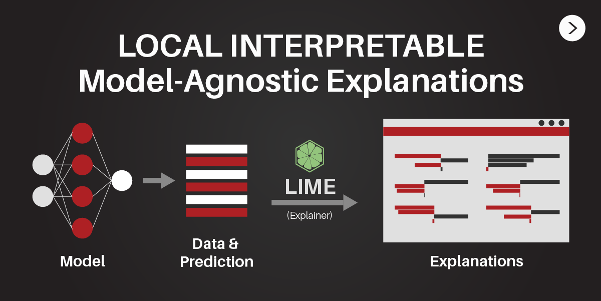
There exist a method called LIME, a novel explanation technique that explains the predictions of any classifier in an interpretable and faithful manner, by learning an interpretable model locally around the prediction. Here we will see how LIME works on text classification problem of user review. By understanding on how our model works, we can have more advantage and could act wiser on what should we do.
Library and Setup
Here is the list of required packages if you wish to reproduce the result.
# Data Wrangling
library(tidyverse)
library(tm)
library(tidytext)
library(textclean)
library(SnowballC)

# Model Fitting and Evaluation
library(caret)
library(e1071)

# Model Interpretation
library(lime)
Use Case: Steam Game Reviews
For this topic, we will cover text mining application to predict customer perspective in Gaming industry. Gaming is a growing entertainment industry that can be enjoyed by everyone, from a little children to the elderly (see a Grandma play Skyrim). Gaming industry has estimated revenue of USD 43.3 Billions, surpassing global ticket sales of Box Office (USD 41.7 Billions) and streaming services (USD 28.8 Billions) in 20181.
Video games come in many platform, such as Wii, Playstation, Xbox, or even in PC. One of the most lucrative gaming environment in PC is Steam, where people can purchase, discuss, or even create games. Many top ranked game are sold via Steam.
The question is, what a review have to do in Gaming industry? It turns out that a game review, especially an early access review, can heavily influence people to buy certain games2. An early access review is a review that is give by people or organization that have played the game in the alpha or beta phase (the unfinished product). Some organization, such as the Polygon, PC Gamer, or Rock Paper Shotgun, has a role to assess and give critics to many games. There are also several individual that give game review and critics in their personal blog or Youtube Channel. They have many loyal reader that trust their reviews. Therefore, any critics given by them will become a great consideration for a player to buy a certain games. However, a review given at the full version release of the game is also important as well. Many late buyer or a skeptic people only buy a game after reading other people review after they play the game.
Through text mining, we can predict based on the given review that a user will give a recommendation toward a game. Further analyisis can be done by interpreting how the machine learning model works and interpret the result. For example, what words that will increase the probability for people to give recommendation, or what words that will drastically decrease the probability to give recommendation. Based on the result, we can formulate a new strategy and marketing planning for future improvement of the game, to make sure people will buy and stay loyal to our game.
Import Data
The data is acquired from Kaggle . It contain reviews from Steam’s best selling games as February 2019.
review <- data.table::fread("data_input/steam_reviews.csv") %>%
  mutate(recommendation = as.factor(recommendation))

glimpse(review)
Data description:
- date_posted: The date of posted review
- funny: How many other player think the review is funny
- helpful: How many other player think the review is helpful
- hour_played: How many hour a reviewer play the game before make a review
- is_early_access_review: Is the game on early access?
- recommendation: Whether the user would recommend the game or not
- review: User review
- title: Title of the game
Exploratory Data Analysis
Before we do model fitting, let’s check the proportion of recommendation based on whether the review is given at the early access or not.
table(Is_early_access = review$is_early_access_review,
      Recommend = review$recommendation) %>%
  prop.table() %>%
  addmargins()
Based on the table, we can see that only 30% of the review come from the early access review. We can choose to only consider the early access review, but for now I will simply use all of the data.
Let’s check the class imbalance at the target variable.
table(review$recommendation) %>%
  prop.table()
Many user tag a game as recommended, with only 30% consider a game is not recommended.
Cross-Validation
Let’s split the data into training set and testing set with 75% of the data will be used as the training dataset.
set.seed(123)
row_review <- nrow(review)
index <- sample(row_review, row_review*0.75)

data_train <- review[ index, ]
data_test <- review[ -index, ]
Check the class proportion on the target variable.
table(data_train$recommendation) %>%
  prop.table()
We will balance the data using down-sampling method. This will increase the model performance.
set.seed(123)
data_train <- downSample(x = data_train$review,
                         y = data_train$recommendation, yname = "recommendation")

table(data_train$recommendation) %>%
  prop.table()
Now we are ready to process the text data.
Text Mining in R
Text mining in R can be done in various way. There are some packages that support text processing. If you are new to text mining, I recommend you to read this wonderfull book . On this article, we will use two approach: tm and a combination of text_clean and tidytext. The difference between the two approach is the preprocessing steps in handling the text data.
Using tm package
The first package that we will use is tm package.
Text Cleansing
We will create a corpus that contain the text review and cleanse the data
review_corpus <- VCorpus( VectorSource(data_train$x))

review_corpus <- review_corpus %>%
  tm_map(content_transformer(tolower)) %>% # lowercase
  tm_map(removeNumbers) %>% # remove numerical character
  tm_map(removeWords, stopwords("english")) %>%  # remove stopwords (and, the, am)
  tm_map(removePunctuation) %>%  # remove punctuation mark
  tm_map(stemDocument) %>%  # stem word (e.g. from walking to walk)
  tm_map(stripWhitespace) # strip double white space
Document Term Matrix
After we cleanse the text, now we will do tokenization: break a sentence or review into an individual words/terms and count the frequency at each document/review.
train_dtm <- DocumentTermMatrix(review_corpus)We have around 196K reviews with 136K unique terms/words.
Filter Terms
Filter words that appear in at least 300 documents to shorten the computation time.
freq <- findFreqTerms(train_dtm, 300)
length(freq)

train_dtm <- train_dtm[ , freq]
We will only use 1584 terms to build the model. You may want to use more terms if you wish.
Bernoulli Converter
Convert the term frequency with bernoulli converter to account binary value (whether the terms present in the document or not).
bernoulli_conv <- function(x){
        x <- factor(
          ifelse(x > 0, 1, 0), levels = c(0,1), labels = c("Absent", "Present")
          )
        return(x)}

# convert the document-term matrix
train_x <- apply(train_dtm, 2, bernoulli_conv)

# create the target variable
train_label <- data_train$recommendation
Model Fitting
We will create a Naive Bayes model to predict the target variable based on the presence of each term. We also use laplace smoothing.
model_bayes <- naiveBayes(train_x, train_label, laplace = 1)Model Evaluation
Before we predict the data, let’s summarize the text preprocessing into a single function and store it as tokenize_text(). This function will be used to clean and tokenize the review from the testing dataset.
tokenize_text <- function(text){
  # Create Corpuse
  data_corpus <- VCorpus(VectorSource(text))

  # Cleansing
  data_corpus_clean <-  data_corpus %>%
    tm_map(content_transformer(tolower)) %>%
    tm_map(removeNumbers) %>%
    tm_map(removeWords, stopwords("english")) %>%
    tm_map(removePunctuation) %>%
    tm_map(stemDocument) %>%
    tm_map(stripWhitespace) %>%
    tm_map(stemDocument)

  # Document-Term Matrix and use only terms from data train
  data_dtm <- DocumentTermMatrix(data_corpus_clean,
                                 control = list(dictionary = freq))

  # Bernoulli Converter
  data_text <- apply(data_dtm, 2, bernoulli_conv)

  return(data_text)
}
Now let’s predict the model performance.
test_x <- tokenize_text(data_test$review)
test_label <- data_test$recommendation

pred_test <- predict(model_bayes, test_x)

confusionMatrix(pred_test, test_label, positive = "Recommended")
The model is quite good, with 73.6% accuracy, 85% Recall and 78% Precision.
Interpret Model with LIME
LIME is a great model that can interpret how our machine learning model (in this case, Naive Bayes) works and make prediction. In R, it come from lime package. However, LIME can only interpret model from several packages, including:
caretmlrxgboosth20kerasMASS
Our model comes from naiveBayes() function from e1071 package, so by default they cannot be identified by lime().
We have to create a support function for the naiveBayes() function in order to be interpreted by LIME. Let’s check the class of our model.
class(model_bayes)
We need to change the class of our model from naiveBayes to either classification or regression (depends on the problem). Since our case is a classification problem, we will change the model type into classification by creating a function.
You have to create a function named model_type. followed by the class of the model. In our model, the class is naiveBayes, so we need to create a function named model_type.naiveBayes.
model_type.naiveBayes <- function(x){
  return("classification")
}
We also need a function to store the prediction. Same with the model_type., we need to create a predict_model. followed by the class of our model. The function would be predict_model.naiveBayes. The content of the function is the function to predict the model. In Naive Bayes, the function is predict(). We need to return the probability value and convert them to data.frame, so the content would be predict(x, newdata, type = "raw") to return the probability of the prediction and convert them with as.data.frame().
predict_model.naiveBayes <- function(x, newdata, type = "raw") {

    # return classification probabilities only
    res <- predict(x, newdata, type = "raw") %>% as.data.frame()

    return(res)
}
Now, we need to prepare the input for the lime. In common classification problem, the input can be the table that contain the features. However, in text classification, the input should be the original text and we also need to give the preprocessing step to process the text from cleansing to the tokenization. Make sure the input of the text is character, not a factor.
text_train <- data_train$x %>% as.character() # The text review from data train

explainer <- lime(text_train, # the input
                  model = model_bayes,  # the model
                  preprocess = tokenize_text) # the preprocessing step
Now we will try to explain how our model work on the test dataset. We will observe the interpretation of the 2nd to 5th obervations of the data test. Don’t forget to do set.seed to get reproducible example.
- The
n_labelsindicate how many label of target variable to be shown. - The
n_featuresshows how many features will be used to explain the model. This parameter will be ignored iffeature_select = "none. - The
feature_selectshows the feature selection method. single_explanationindicate logical whether to pool all text into a single review.
text_test <- data_test$review

set.seed(123)
explanation <- explain(text_test[2:5],
                       explainer = explainer,
                       n_labels = 1, # show only 1 label (recommend or not recommend)
                       n_features = 5,
                       feature_select = "none", # use all terms to explain the model
                       single_explanation = F)
Let’s visualize the result.
# visualize the interpretation
plot_text_explanations(explanation)

Since the plot is run from a chunk, the output height and width of the plot is limited. If you want to scroll or see the complete plot, you need to run the plot_text_explanations() via the console.
We can see that for observations 2 (the first sentence), the probability to be not recommended is 100%. The explanation fit shows how good LIME at interpreting the prediction for this observation, which is only 27% so it may not that accurate. The blue-labeled text means that the word support/increase the probability to be not recommend, such as the word game, start or long time. The red-labeled text means that the word contradict/decrease the probability of the review to be recommended, such as fun, most infuriating or powerful.
The interpretation is not that good since the explanation fit is small, but at least we can derive some insight from it. We can also observe from the second sentenct that the word difficult, gast, and Materpiece contradict the probability to be not recommended.
A good example of great explanation fit is at the 3rd text (observation 4), with explanation fit of 80%. We can see that the word glitch, bug and error can support the review to be not recommended.
Using textclean
Another great package for text processing is textclean package. You can read more detail about it on our previous article .
Data Preprocessing
We will use the same data from the previous process. Using text_clean, we create a new column that contain the processed text that will be cleansed using various functions from the package.
data_train <- data_train %>%
  mutate(text_clean = x %>%
            str_to_lower() %>%
            replace_url() %>%
            replace_money(replacement = "") %>%
            replace_emoji() %>%
            replace_email() %>%
            replace_word_elongation() %>%
            replace_html() %>%
            replace_contraction() %>%
            replace_number(remove = T) %>%
            replace_date(replacement = "") %>%
            str_remove_all(pattern = "[[:punct:]]") %>%
            str_squish() %>%
            str_trim()
           )

head(data_train, 10)
Document-Term Matrix
After we cleanse the data, next we will need to tokenize the data by converting it into document-term matrix.
train_dtm <- data_train %>%
  select(text_clean, recommendation) %>%
  rowid_to_column("id") %>%
  filter(is.na(text_clean) == F) %>%
  unnest_tokens(word, text_clean) %>%
  mutate(word = wordStem(word)) %>%
  anti_join(stop_words) %>%
  count(id, word) %>%
  cast_dtm(document = id, term = word, value = n)

inspect(train_dtm)
Let’s use terms that appear at least in 200 documents.
train_term <- findFreqTerms(train_dtm, 200)
length(train_term)
Next we use bernoulli converter toward the document-term matrix. We will also get the train label.
# Filter the terms in DTM
train_dtm <- train_dtm[ , train_term]

# Apply bernoulli converter
train_x <- apply(train_dtm, 2, bernoulli_conv)

# Create train label
train_label <- data_train %>%
  slice(  as.numeric(train_dtm$dimnames$Docs)) %>%
  pull(recommendation)
Model Fitting
We fit the data into the Naive Bayes model with laplace smoothing.
model_bayes <- naiveBayes(train_x, train_label, laplace = 1)Model Evaluation
Next, we evaluate the model to the testing dataset. We summarise the preprocessing step into a single function and store it as tokenize_text().
tokenize_text <- function(text){
 clean_text <-  text %>%
    str_to_lower() %>%
    replace_url() %>%
    replace_emoji() %>%
    replace_email() %>%
    replace_word_elongation() %>%
    replace_html() %>%
    replace_contraction() %>%
    replace_number(remove = T) %>%
    replace_date() %>%
    str_remove_all(pattern = "[[:punct:]]") %>%
    str_squish() %>%
    str_trim()

  data_text <- data.frame(text_clean = clean_text) %>%
    rowid_to_column("id") %>%
    filter(is.na(text_clean) == F) %>%
    mutate_all(as.character) %>%
    unnest_tokens(word, text_clean) %>%
    mutate(word = wordStem(word)) %>%
    filter(word %in% train_term) %>% # Use only terms that appear in training set
    count(id, word) %>%
    cast_dtm(document = id, term = word, value = n) %>%
    apply(., 2, bernoulli_conv)

  return(data_text)
}

# tokenize text review
test_x <- tokenize_text(data_test$review)

# get target variable
test_label <- data_test %>%
  slice(
    as.numeric( test_x %>% rownames() )
    ) %>%
  pull(recommendation)
After we prepare the data, now we will predict the target for the testing dataset and acquire the confusion matrix.
pred_test <- predict(model_bayes, test_x)

confusionMatrix(pred_test, test_label, positive = "Recommended")
Interpret model with LIME
To interpret the model with LIME, the step is similar to the one we’ve done by using the tm package. The difference is only the preprocessing step, tokenize_text(). To make the computation faster, we can adjust the number of permutations performed by lime through parameter n_permutations. On the following example, I use n_permutations of 10. Don’t forget to do set.seed to get reproducible example.
# Get text review from training set
train_text <- data_train %>%
  slice(
    as.numeric( train_x %>% rownames() )
    ) %>%
  pull(x) %>% as.character()

# Get text review from testing set
test_text <- data_test$review

# Set explainer
explainer <- lime(train_text, model_bayes,
                  preprocess = tokenize_text)

set.seed(111)
explanation <- explain(test_text[2:5],
                       explainer, n_labels = 1,
                       n_features = 5,
                       n_permutations = 10, # Adjust the number of permutation
                       feature_select = "none",
                       single_explanation = F)
Let’s visualize the result.
# Plot the visualization
plot_text_explanations(explanation)

Error and Troubleshoot
This section is dedicated to give some insight from potential error that you might find when using lime.
Response is constant across permutations
You may wonder why we don’t insert the first observation of the review to the explanation. Let’s check the review content.
data_test$review[1]The review containt only the word “yes”. We will try to explain it with LIME. Since the explainer expect a matrix, we need to insert at least 2 observations, so will go with the first and the second observation.
set.seed(123)
explanation <- explain(test_text[1:2],
                       explainer = explainer,
                       n_labels = 1, # show only 1 label (recommend or not recommend)
                       n_features = 5,
                       n_permutations = 10,
                       feature_select = "none", # use all terms to explain the model
                       single_explanation = F)
We get an error, with message Error: Response is constant across permutations. Please check your model. One of many reason it throws an error is because the input for our model is a document-term matrix, with many sparse/empty values. LIME don’t work really with an input that contain many sparse value like in text classification3. With the text contain only the word yes, the matrix will be 0 (Absent) or sparse for most of the feature and 1 (Present) for a single feature, that is the term yes. So, whenever you found an error like this, you can be certain that the input is a matrix with empty values. To my best knowledge, there is no workaround for this problem yet. Therefore, we only concern with a review or text that contain several words.
Predicted_label is not a string (a length one character vector)
If we want to use the plot_text_explanations(), the n_labels should always be 1, meaning that we can only display output for 1 label or target value, either the Recommended or Not Recommended. If you force the explainer to include 2 labels, it will give an error like the following.
set.seed(123)
explanation <- explain(test_text[2:3],
                       explainer = explainer,
                       n_labels = 2, # show 2 label (recommend or not recommend)
                       n_features = 5,
                       n_permutations = 10,
                       feature_select = "none", # use all terms to explain the model
                       single_explanation = F)

plot_text_explanations(explanation)
Incorrect number of predictions
Whenever you find an error, you can look at the cause of the error by using traceback() function. Here is another example of error.
set.seed(123)
explanation <- explain(test_text[2:4],
                       explainer = explainer,
                       n_labels = 1, # show only 1 label (recommend or not recommend)
                       n_features = 5,
                       n_permutations = 10,
                       feature_select = "none", # use all terms to explain the model
                       single_explanation = F)
traceback()The traceback() will return the following result.
# 4: stop(assertError(attr(res, "msg")))
# 3: assert_that(nrow(case_res) == length(case_perm$permutations),
#        msg = "Incorrect number of predictions")
# 2: explain.character(test_text[2:4], explainer, n_labels = 1, n_features = 5,
#        n_permutations = 10, feature_select = "none", single_explanation = F)
# 1: explain(test_text[2:4], explainer, n_labels = 1, n_features = 5,
#        n_permutations = 10, feature_select = "none", single_explanation = F)
Based on the traceback result, explain() is error because the number of row for the predicted values (case_res) is not the same with the length of the permutation (case_perm$permutations). You can check the source code ) to see what really happened, but based on the error, the permutation failed to produce a prediction, therefore we have less number of prediction compared to the number of permutation. Since a permutation is a sampling problem, for temporary solution you can handle the problem by changing the seed for the explanation or simply change the number of permutation via n_permutations.
Conclusion
LIME is very useful to help us understand how our model works not only in a common classification problem with the feature presented in tabular format, but it can also interpret how the model work by looking at the text-formatted input. The important point of using lime is you have to define how the text is preprocessed until it can become a matrix as the input for the model. I also have shown you several errors that may shows up when you try to use LIME.
 More details
 More details
Share this post
Twitter
Facebook
LinkedIn