

Introduction
Deep learning is a great approach to deal with unstructured data such as text, sound, video and image. There are a lot of implementation of deep learning in image classification and image detection, such as classifying image of dog or cats, detecting different objects in an image or do facial recognition.
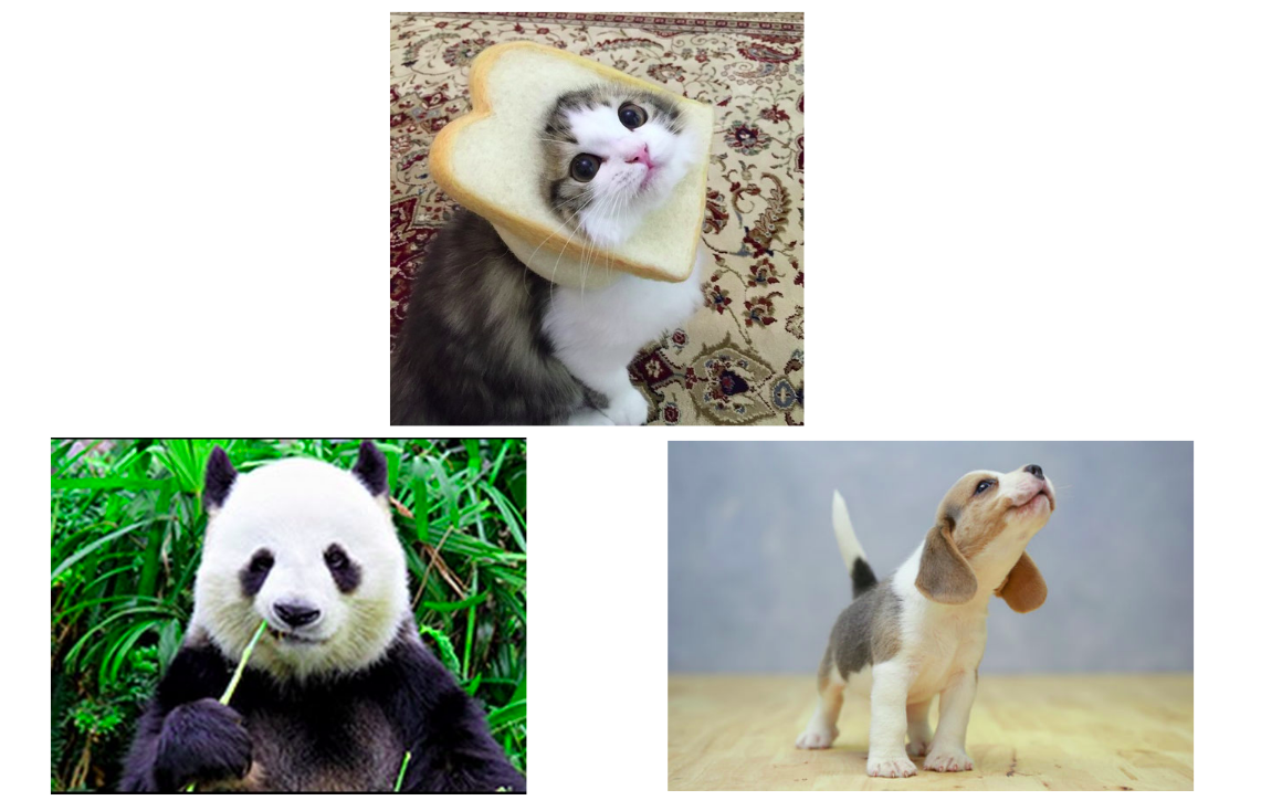
On this article, we will try to build a simple image classification that will classify whether the presented image is a cat, dog, or a panda.
Data
You can download the data and the source code for practice here. The data is a modified version the Animal Image Dataset(DOG, CAT and PANDA) on Kaggle.
Library and Setup
You need to install the pillow package in your conda environment to manipulate image data. Here is the short instruction on how to create a new conda environment with tensorflow and pillow inside it.
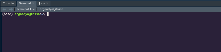
- Open the terminal, either in anaconda command prompt or directly in RStudio.
- Create new conda environment by running the following command.
conda create -n tf_image python=3.7
- Active the conda environment by running the following command.
conda activate tf_image
- Install the tensorflow package into the environment.
conda install -c conda-forge tensorflow=2
- Install the
pillowpackage.
pip install pillow
- The next step is just call your conda environment using
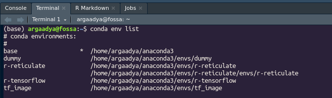
reticulate::use_python()and insert the location of the python from thetf_imageenvironment. You can locate the path or the location of the environment by typingconda env listin the terminal.
# Use python in your anaconda3 environment folder
reticulate::use_python("~/anaconda3/envs/tf_image/bin/python", required = T)
The following is the list of required packages to build and evaluate our image classification.
# Data wrangling
library(tidyverse)

# Image manipulation
library(imager)

# Deep learning
library(keras)

# Model Evaluation
library(caret)

options(scipen = 999)
Exploratory Data Analysis
Let’s explore the data first before building the model. In image classification problem, it is a common practice to put each image on separate folders based on the target class/labels. For example, inside the train folder in our data, you can that we have 3 different folders, respectively for cats, dogs, and panda.
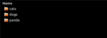
If you open the cat folder, you can see that we have no table or any kind of structured data format, we only have the image for the cat. We will directly extract information from the images instead of using a structured dataset.
Let’s try to get the file name of each image. First, we need to locate the folder of each target class. The following code will give you the folder name inside the train folder.
folder_list <- list.files("data_input/image_class/train/")

folder_list
#> [1] "cats" "dogs" "panda"We combine the folder name with the path or directory of the train folder in order to access the content inside each folder.
folder_path <- paste0("data_input/image_class/train/", folder_list, "/")

folder_path
#> [1] "data_input/image_class/train/cats/" "data_input/image_class/train/dogs/"
#> [3] "data_input/image_class/train/panda/"We will use the map() function to loop or iterate and collect the file name for each folder (cat, dog, panda). The map() will return a list so if we want to combine the file name from 3 different folders we simply use the unlist() function.
# Get file name
file_name <- map(folder_path,
                 function(x) paste0(x, list.files(x))
                 ) %>%
  unlist()

# first 6 file name
head(file_name)
#> [1] "data_input/image_class/train/cats/cats_001.jpg"
#> [2] "data_input/image_class/train/cats/cats_002.jpg"
#> [3] "data_input/image_class/train/cats/cats_003.jpg"
#> [4] "data_input/image_class/train/cats/cats_004.jpg"
#> [5] "data_input/image_class/train/cats/cats_005.jpg"
#> [6] "data_input/image_class/train/cats/cats_006.jpg"You can also check the last 6 images.
# last 6 file name
tail(file_name)
#> [1] "data_input/image_class/train/panda/panda_00994.jpg"
#> [2] "data_input/image_class/train/panda/panda_00995.jpg"
#> [3] "data_input/image_class/train/panda/panda_00996.jpg"
#> [4] "data_input/image_class/train/panda/panda_00997.jpg"
#> [5] "data_input/image_class/train/panda/panda_00998.jpg"
#> [6] "data_input/image_class/train/panda/panda_00999.jpg"Let’s check how many images we have.
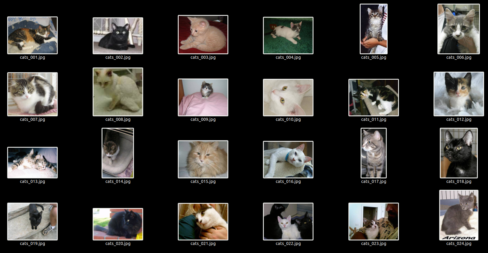
length(file_name)#> [1] 2659To check the content of the file, we can use the load.image() function from the imager package. For example, let’s randomly visualize 6 images from the data.
# Randomly select image
set.seed(99)
sample_image <- sample(file_name, 6)

# Load image into R
img <- map(sample_image, load.image)

# Plot image
par(mfrow = c(2, 3)) # Create 2 x 3 image grid
map(img, plot)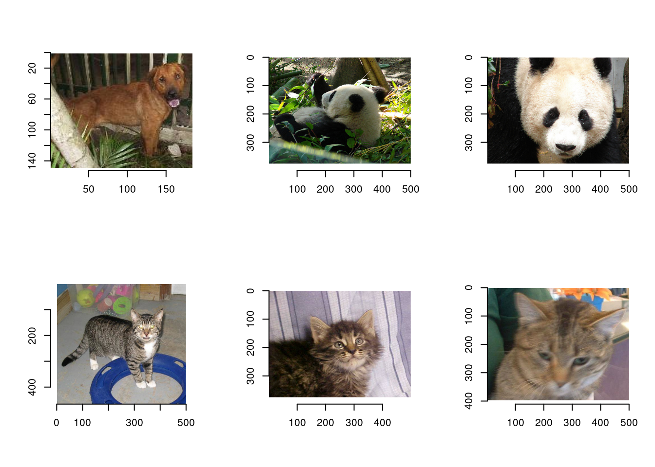
#> [[1]]
#> Image. Width: 184 pix Height: 149 pix Depth: 1 Colour channels: 3
#>
#> [[2]]
#> Image. Width: 500 pix Height: 375 pix Depth: 1 Colour channels: 3
#>
#> [[3]]
#> Image. Width: 500 pix Height: 375 pix Depth: 1 Colour channels: 3
#>
#> [[4]]
#> Image. Width: 500 pix Height: 466 pix Depth: 1 Colour channels: 3
#>
#> [[5]]
#> Image. Width: 499 pix Height: 375 pix Depth: 1 Colour channels: 3
#>
#> [[6]]
#> Image. Width: 500 pix Height: 397 pix Depth: 1 Colour channels: 3
Check Image Dimension
One of important aspects of image classification is understand the dimension of the input images. You need to know the distribution of the image dimension to create a proper input dimension for building the deep learning model. Let’s check the properties of the first image.
# Full Image Description
img <- load.image(file_name[1])
img
#> Image. Width: 499 pix Height: 375 pix Depth: 1 Colour channels: 3You can get the information about the dimension of the image. The height and width represent the height and width of the image in pixels. The color channel represent if the color is in grayscale format (color channels = 1) or is in RGB format (color channels = 3). To get the value of each dimension, we can use the dim() function. It will return the height, width, depth, and the channels.
# Image Dimension
dim(img)
#> [1] 499 375 1 3So we have successfully insert an image and get the image dimensions. On the following code, we will create a function that will instantly get the height and width of an image and convert it into a data.frame.
# Function for acquiring width and height of an image
get_dim <- function(x){
  img <- load.image(x)

  df_img <- data.frame(height = height(img),
                       width = width(img),
                       filename = x
                       )

  return(df_img)
}

get_dim(file_name[1])
#> height width filename
#> 1 375 499 data_input/image_class/train/cats/cats_001.jpgNow we will sampling 1,000 images from the file name and get the height and width of the image. We use sampling here because it will take a quite long time to load all images.
# Randomly get 1000 sample images
set.seed(123)
sample_file <- sample(file_name, 1000)

# Run the get_dim() function for each image
file_dim <- map_df(sample_file, get_dim)

head(file_dim, 10)
#> height width filename
#> 1 375 500 data_input/image_class/train/panda/panda_00780.jpg
#> 2 375 500 data_input/image_class/train/panda/panda_00836.jpg
#> 3 375 500 data_input/image_class/train/panda/panda_00521.jpg
#> 4 294 363 data_input/image_class/train/cats/cats_526.jpg
#> 5 269 172 data_input/image_class/train/cats/cats_195.jpg
#> 6 375 500 data_input/image_class/train/panda/panda_00072.jpg
#> 7 255 234 data_input/image_class/train/dogs/dogs_00313.jpg
#> 8 499 375 data_input/image_class/train/dogs/dogs_00450.jpg
#> 9 374 500 data_input/image_class/train/dogs/dogs_00466.jpg
#> 10 500 440 data_input/image_class/train/dogs/dogs_00187.jpgNow let’s get the statistics for the image dimensions.
summary(file_dim)#> height width filename
#> Min. : 50.0 Min. : 59.0 Length:1000
#> 1st Qu.: 331.0 1st Qu.: 350.0 Class :character
#> Median : 375.0 Median : 499.0 Mode :character
#> Mean : 368.2 Mean : 425.4
#> 3rd Qu.: 411.2 3rd Qu.: 500.0
#> Max. :1023.0 Max. :1024.0The image data has a great variation in the dimension. Some images has less than 60 pixels in height and width while others has up to 1024 pixels. Understanding the dimension of the image will help us on the next part of the process: data preprocessing.
Data Preprocessing
Data preprocessing for image is pretty simple and can be done in a single step in the following section.
Data Augmentation
Based on our previous summary of the image dimensions, we can determine the input dimension for the deep learning model. All input images should have the same dimensions. Here, we can determine the input size for the image, for example transform all image into 64 x 64 pixels. This process will be similar to us resizing the image. You can use other choice of image dimensions, such as 125 x 125 pixels or even 200 x 200 pixels. Bigger dimensions will have more features but will also take longer time to train. However, if the image size is too small, we will lose a lot of information from the data. So balancing this trade-off is the art of data preprocessing in image classification.
We also set the batch size for the data so the model will be updated every time it finished training on a single batch. Here, we set the batch size to 32.
# Desired height and width of images
target_size <- c(64, 64)

# Batch size for training the model
batch_size <- 32
Since we have a little amount of training set, we will build artificial data using method called Image Augmentation. Image augmentation is one useful technique in building models that can increase the size of the training set without acquiring new images. The goal is that to teach the model not only with the original image but also the modification of the image, such as flipping the image, rotate it, zooming, crop the image, etc. This will create more robust model. We can do data augmentation by using the image data generator from keras.
To do image augmentation, we can fit the data into a generator. Here, we will create the image generator for keras with the following properties:
- Scaling the pixel value by dividing the pixel value by 255
- Flip the image horizontally
- Flip the image vertically
- Rotate the image from 0 to 45 degrees
- Zoom in or zoom out by 25% (zoom 75% or 125%)
- Use 20% of the data as validation dataset
You can explore more features about the image generator on this link.
# Image Generator
train_data_gen <- image_data_generator(rescale = 1/255, # Scaling pixel value
                                       horizontal_flip = T, # Flip image horizontally
                                       vertical_flip = T, # Flip image vertically
                                       rotation_range = 45, # Rotate image from 0 to 45 degrees
                                       zoom_range = 0.25, # Zoom in or zoom out range
                                       validation_split = 0.2 # 20% data as validation data
                                       )
Now we can insert our image data into the generator using the flow_images_from_directory(). The data is located inside the data folder and inside the train folder, so the directory will be data/train. From this process, we will get the augmented image both for training data and the validation data.
# Training Dataset
train_image_array_gen <- flow_images_from_directory(directory = "data_input/image_class/train/", # Folder of the data
                                                    target_size = target_size, # target of the image dimension (64 x 64)
                                                    color_mode = "rgb", # use RGB color
                                                    batch_size = batch_size ,
                                                    seed = 123,  # set random seed
                                                    subset = "training", # declare that this is for training data
                                                    generator = train_data_gen
                                                    )

# Validation Dataset
val_image_array_gen <- flow_images_from_directory(directory = "data_input/image_class/train/",
                                                  target_size = target_size,
                                                  color_mode = "rgb",
                                                  batch_size = batch_size ,
                                                  seed = 123,
                                                  subset = "validation", # declare that this is the validation data
                                                  generator = train_data_gen
                                                  )
Here we will collect some information from the generator and check the class proportion of the train dataset. The index correspond to each labels of the target variable and ordered alphabetically (cat, dog, panda).
# Number of training samples
train_samples <- train_image_array_gen$n

# Number of validation samples
valid_samples <- val_image_array_gen$n

# Number of target classes/categories
output_n <- n_distinct(train_image_array_gen$classes)

# Get the class proportion
table("\nFrequency" = factor(train_image_array_gen$classes)
      ) %>%
  prop.table()
#>
#> Frequency
#> 0 1 2
#> 0.3344293 0.3363081 0.3292626Convolutional Neural Network
The Convolutional Neural Network or Convolutional Layer is a popular layer for image classification. If you remember, an image is just a 2 dimensional array with certain height and width. For example, an image with 64 x 64 pixels means that it has 4096 pixels that is distributed in a 64 x 64 array instead of a single dimensional vector. The benefit of using image as a 2D array is that we can extract certain features from the image such as the shape of nose, the shape of eyes, hand, etc.
Take the following amazing example from setosa.io. We have an image and its 2D array representation. The value on the array is the pixel value from the image, higher value means brighter pixel.
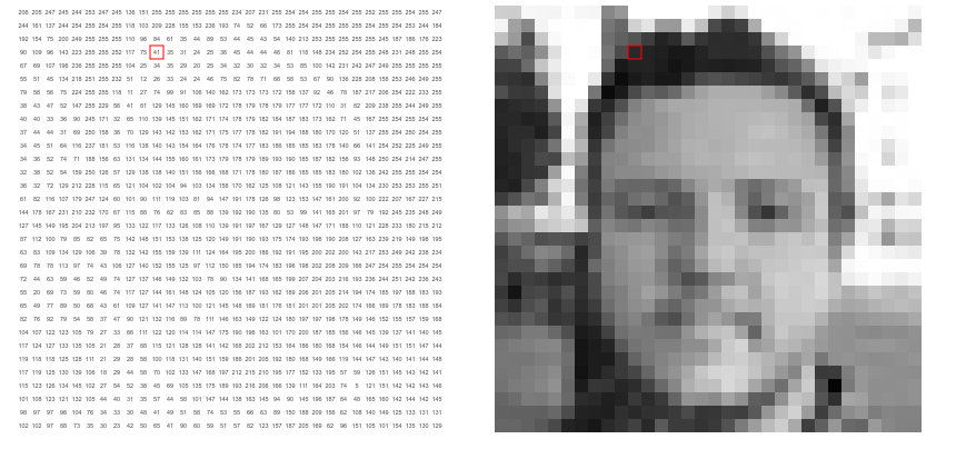
To extract features from the image, we create something called a filter kernel. A filter is an array with certain size, for example 3 x 3 array to capture features from image. In the following figure, the rectangle illustrated a single filter kernel.
For example, the left side of the following picture is a 5 x 5 images. The kernel has a weight that will capture certain features, which in this example is an X features that indicated by the value of 1 create an X shape. The new convoluted feature is the product of the image section with the kernel feature. The more similar image section with the kernel, the higher the score of the convoluted feature.
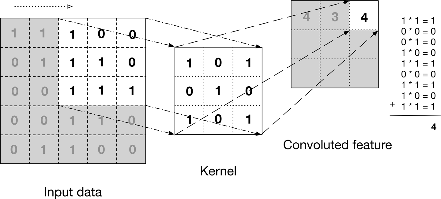
The kernel wil move sideway to the right to capture each section of the image to create new convoluted feature. If the kerel has reach the edge, it will go down 1 row below and continue the process. The process is illustrated as follows. Visit stanford course on Convolutional Neural Network for more info about the figure and other info.
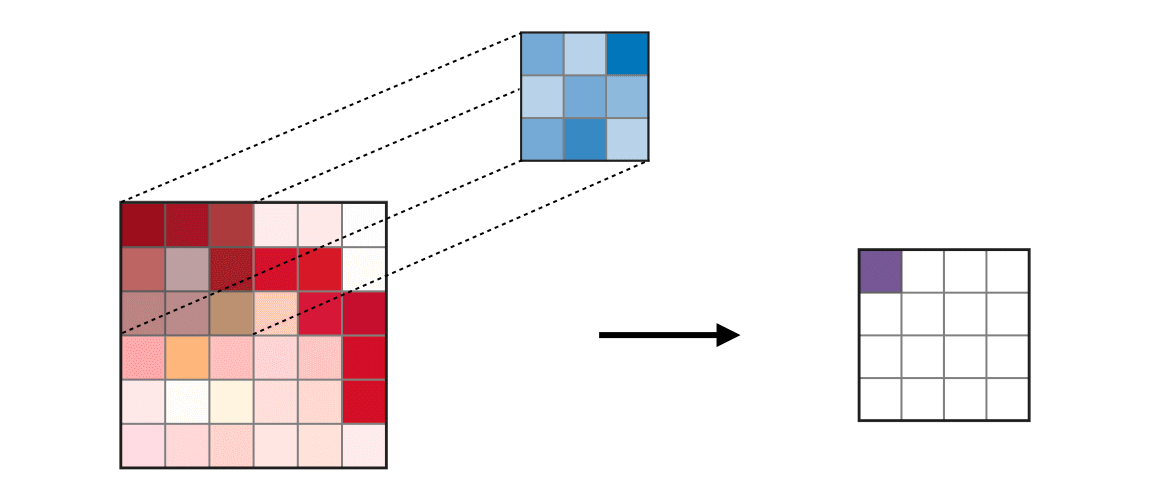
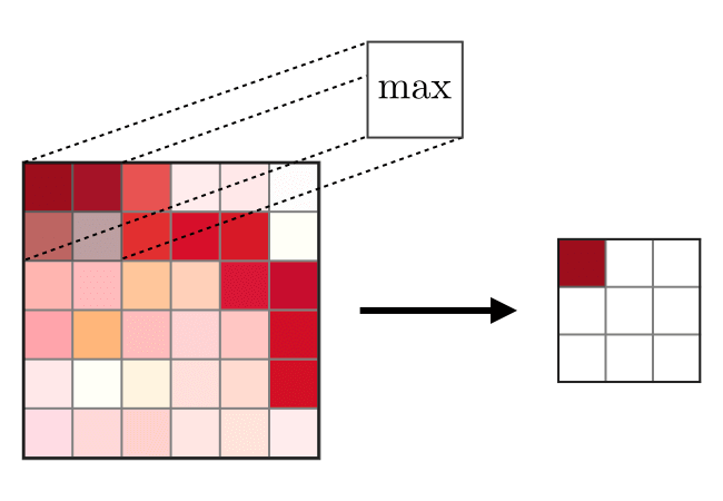
To highglight the most important feature and also downsize the dimension of the convoluted feature, we can use a method called the Max pooling which take only the maximum value from certain window. For example, in the top left array that contains the value of 1, 1, 5, and 6, it only take the max value, which is 6.
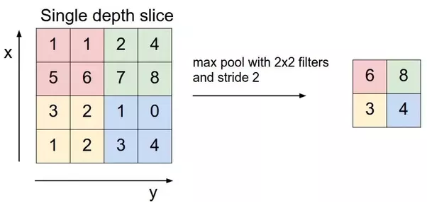
Below is the illustration of doing max pooling of 2 x 2 pooling area along the sections. Max pooling only take the maximum value of each pooling area.
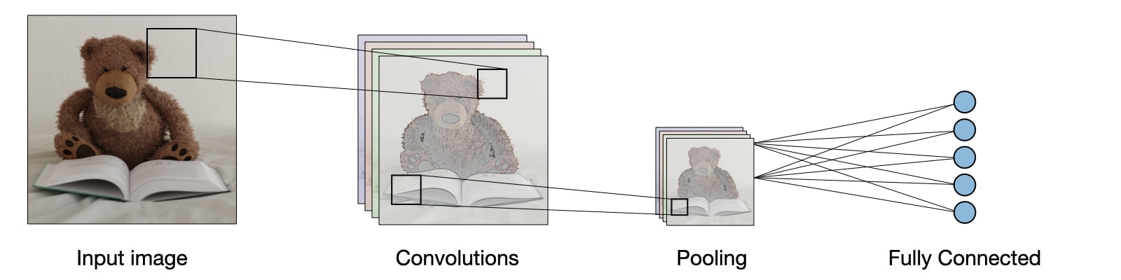
To make the extracted 2D array into a 1D array, we use the flattening layer so we can continue using the fully-connected dense layer and to the output layer.
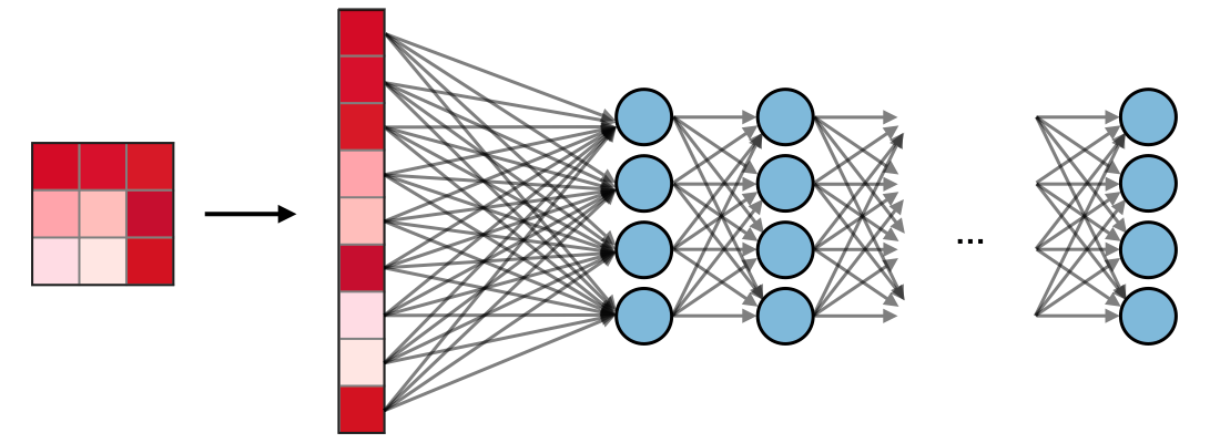
The following figure illustrate the full deep learning model with CNN, max pooling and fully connected dense layer.
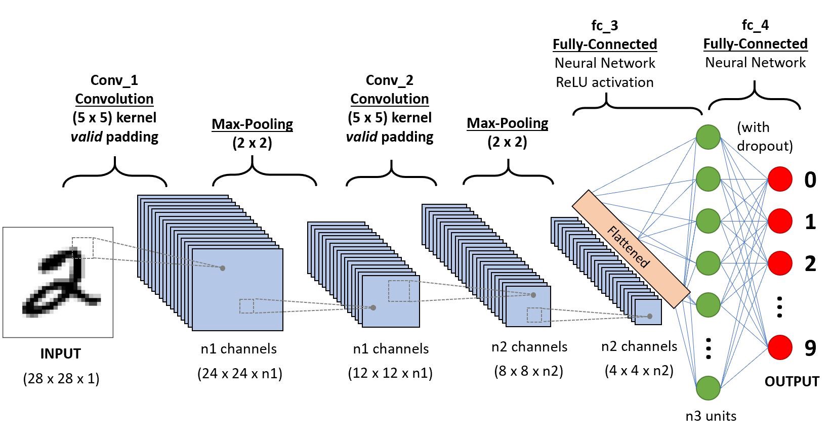
You can see the explanation from MIT for introduction to Deep Learning and Convolutional Neural Network on the deeper level.
Model Architecture
We can start building the model architecture for the deep learning. We will build a simple model first with the following layer:
- Convolutional layer to extract features from 2D image with
reluactivation function - Max Pooling layer to downsample the image features
- Flattening layer to flatten data from 2D array to 1D array
- Dense layer to capture more information
- Dense layer for output with
softmaxactivation function
Don’t forget to set the input size in the first layer. If the input image is in RGB, set the final number to 3, which is the number of color channels. If the input image is in grayscale, set the final number to 1.
# input shape of the image
c(target_size, 3)
#> [1] 64 64 3# Set Initial Random Weight
tensorflow::tf$random$set_seed(123)
model <- keras_model_sequential(name = "simple_model") %>%
# Convolution Layer
layer_conv_2d(filters = 16,
kernel_size = c(3,3),
padding = "same",
activation = "relu",
input_shape = c(target_size, 3)
) %>%
# Max Pooling Layer
layer_max_pooling_2d(pool_size = c(2,2)) %>%
# Flattening Layer
layer_flatten() %>%
# Dense Layer
layer_dense(units = 16,
activation = "relu") %>%
# Output Layer
layer_dense(units = output_n,
activation = "softmax",
name = "Output")
model#> Model
#> Model: "simple_model"
#> ________________________________________________________________________________
#> Layer (type) Output Shape Param #
#> ================================================================================
#> conv2d (Conv2D) (None, 64, 64, 16) 448
#> ________________________________________________________________________________
#> max_pooling2d (MaxPooling2D) (None, 32, 32, 16) 0
#> ________________________________________________________________________________
#> flatten (Flatten) (None, 16384) 0
#> ________________________________________________________________________________
#> dense (Dense) (None, 16) 262160
#> ________________________________________________________________________________
#> Output (Dense) (None, 3) 51
#> ================================================================================
#> Total params: 262,659
#> Trainable params: 262,659
#> Non-trainable params: 0
#> ________________________________________________________________________________As you can see, we start by entering image data with 64 x 64 pixels into the convolutional layer, which has 16 filters to extract featuers from the image. The padding = same argument is used to keep the dimension of the feature to be 64 x 64 pixels after being extracted. We then downsample or only take the maximum value for each 2x2 pooling area so the data now only has 32 x 32 pixels with from 16 filters. After that, from 32 x 32 pixels we flatten the 2D array into a 1D array with 32 x 32 x 16 = 16384 nodes. We can further extract information using the simple dense layer and finished by flowing the information into the output layer, which will be transformed using the softmax activation function to get the probability of each class as the output.
Model Fitting
You can start fitting the data into the model. Don’t forget to compile the model by specifying the loss function and the optimizer. For starter, we will use 30 epochs to train the data. For multilabel classification, we will use categorical cross-entropy as the loss function. For this example, we use adam optimizer with learning rate of 0.01. We will also evaluate the model with the validation data from the generator.
model %>%
  compile(
    loss = "categorical_crossentropy",
    optimizer = optimizer_adam(lr = 0.01),
    metrics = "accuracy"
  )

# Fit data into model
history <- model %>%
  fit(
  # training data
  train_image_array_gen,

  # training epochs
  steps_per_epoch = as.integer(train_samples / batch_size),
  epochs = 30,

  # validation data
  validation_data = val_image_array_gen,
  validation_steps = as.integer(valid_samples / batch_size)
)

plot(history)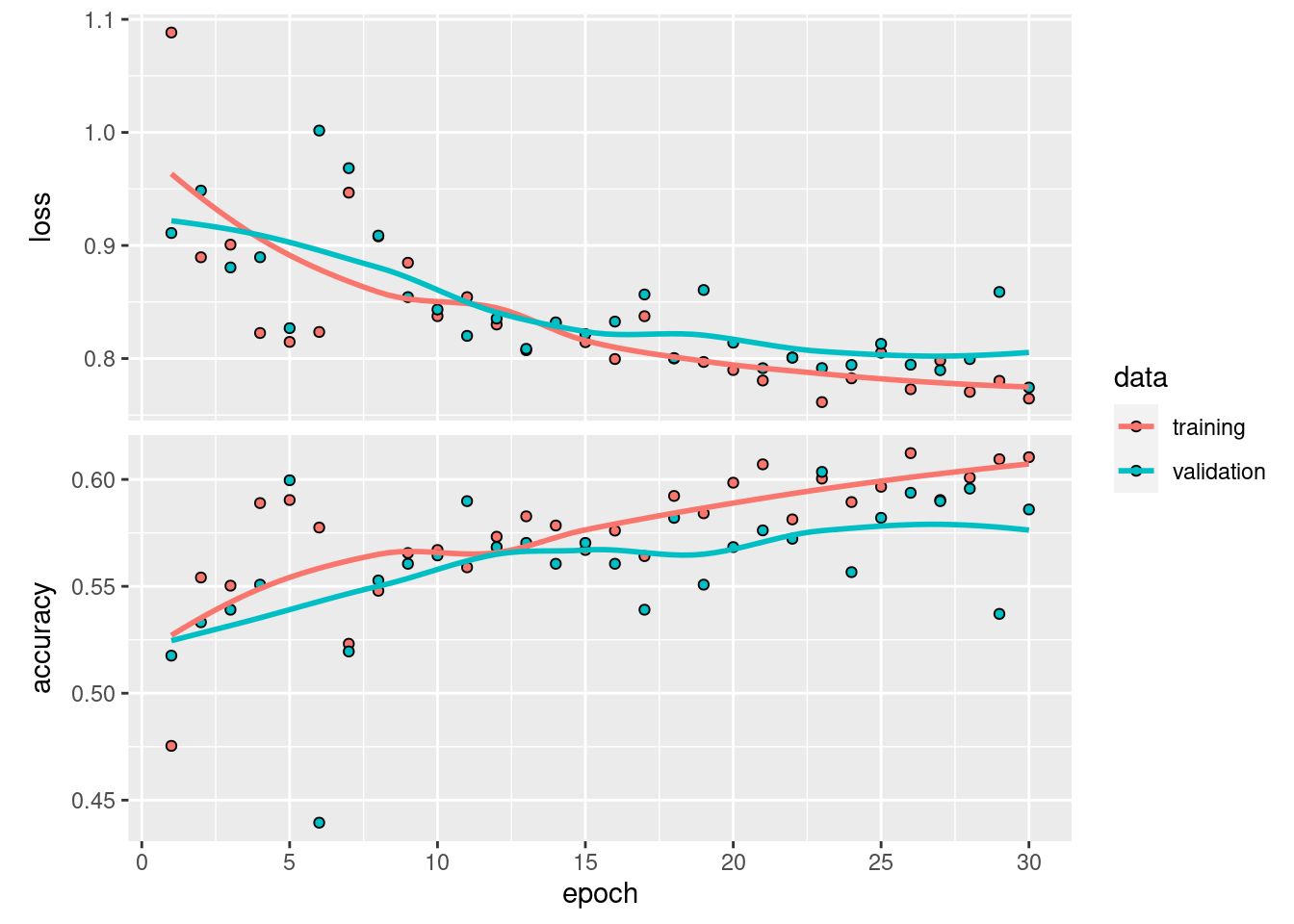
Model Evaluation
Now we will further evaluate and acquire the confusion matrix using the validation data from the generator. First, we need to acquire the file name of the image that is used as the data validation. From the file name, we will extract the categorical label as the actual value of the target variable.
val_data <- data.frame(file_name = paste0("data_input/image_class/train/", val_image_array_gen$filenames)) %>%
  mutate(class = str_extract(file_name, "cat|dog|panda"))

head(val_data, 10)
#> file_name class
#> 1 data_input/image_class/train/cats/cats_001.jpg cat
#> 2 data_input/image_class/train/cats/cats_002.jpg cat
#> 3 data_input/image_class/train/cats/cats_003.jpg cat
#> 4 data_input/image_class/train/cats/cats_004.jpg cat
#> 5 data_input/image_class/train/cats/cats_005.jpg cat
#> 6 data_input/image_class/train/cats/cats_006.jpg cat
#> 7 data_input/image_class/train/cats/cats_007.jpg cat
#> 8 data_input/image_class/train/cats/cats_008.jpg cat
#> 9 data_input/image_class/train/cats/cats_009.jpg cat
#> 10 data_input/image_class/train/cats/cats_010.jpg catWhat to do next? We need to get the image into R by converting the image into an array. Since our input dimension for CNN model is image with 64 x 64 pixels with 3 color channels (RGB), we will do the same with the image of the testing data. The reason of using array is that we want to predict the original image fresh from the folder so we will not use the image generator since it will transform the image and does not reflect the actual image.
# Function to convert image to array
image_prep <- function(x) {
  arrays <- lapply(x, function(path) {
    img <- image_load(path, target_size = target_size,
                      grayscale = F # Set FALSE if image is RGB
                      )

    x <- image_to_array(img)
    x <- array_reshape(x, c(1, dim(x)))
    x <- x/255 # rescale image pixel
  })
  do.call(abind::abind, c(arrays, list(along = 1)))
}
test_x <- image_prep(val_data$file_name)
# Check dimension of testing data set
dim(test_x)#> [1] 530 64 64 3The validation data consists of 530 images with dimensions of 64 x 64 pixels and 3 color channels (RGB). After we have prepared the data test, we now can proceed to predict the label of each image using our CNN model.
pred_test <- predict_classes(model, test_x)

head(pred_test, 10)
#> [1] 1 0 0 2 1 2 0 0 0 0To get easier interpretation of the prediction, we will convert the encoding into proper class label.
# Convert encoding to label
decode <- function(x){
  case_when(x == 0 ~ "cat",
            x == 1 ~ "dog",
            x == 2 ~ "panda"
            )
}

pred_test <- sapply(pred_test, decode)

head(pred_test, 10)
#> [1] "dog" "cat" "cat" "panda" "dog" "panda" "cat" "cat" "cat"
#> [10] "cat"Finally, we evaluate the model using the confusion matrix. The model perform very poorly with low accuracy. We will tune the model by improving the model architecture.
confusionMatrix(as.factor(pred_test),
                as.factor(val_data$class)
                )
#> Confusion Matrix and Statistics
#>
#> Reference
#> Prediction cat dog panda
#> cat 65 48 1
#> dog 42 51 7
#> panda 70 79 167
#>
#> Overall Statistics
#>
#> Accuracy : 0.534
#> 95% CI : (0.4905, 0.5771)
#> No Information Rate : 0.3358
#> P-Value [Acc > NIR] : < 0.00000000000000022
#>
#> Kappa : 0.3023
#>
#> Mcnemar's Test P-Value : < 0.00000000000000022
#>
#> Statistics by Class:
#>
#> Class: cat Class: dog Class: panda
#> Sensitivity 0.3672 0.28652 0.9543
#> Specificity 0.8612 0.86080 0.5803
#> Pos Pred Value 0.5702 0.51000 0.5285
#> Neg Pred Value 0.7308 0.70465 0.9626
#> Prevalence 0.3340 0.33585 0.3302
#> Detection Rate 0.1226 0.09623 0.3151
#> Detection Prevalence 0.2151 0.18868 0.5962
#> Balanced Accuracy 0.6142 0.57366 0.7673Tuning the Model
Model Architecture
Let’s look back at our model architecture. If you have noticed, we can actually extract more information while the data is still in an 2D image array. The first CNN only extract the general features of our image and then being downsampled using the max pooling layer. Even after pooling, we still have 32 x 32 array that has a lot of information to extract before flattening the data. Therefore, we can stacks more CNN layers into the model so there will be more information to be captured. We can also put 2 CNN layers consecutively before doing max pooling.
model#> Model
#> Model: "simple_model"
#> ________________________________________________________________________________
#> Layer (type) Output Shape Param #
#> ================================================================================
#> conv2d (Conv2D) (None, 64, 64, 16) 448
#> ________________________________________________________________________________
#> max_pooling2d (MaxPooling2D) (None, 32, 32, 16) 0
#> ________________________________________________________________________________
#> flatten (Flatten) (None, 16384) 0
#> ________________________________________________________________________________
#> dense (Dense) (None, 16) 262160
#> ________________________________________________________________________________
#> Output (Dense) (None, 3) 51
#> ================================================================================
#> Total params: 262,659
#> Trainable params: 262,659
#> Non-trainable params: 0
#> ________________________________________________________________________________The following is our improved model architecture:
- 1st Convolutional layer to extract features from 2D image with
reluactivation function - 2nd Convolutional layer to extract features from 2D image with
reluactivation function - Max pooling layer
- 3rd Convolutional layer to extract features from 2D image with
reluactivation function - Max pooling layer
- 4th Convolutional layer to extract features from 2D image with
reluactivation function - Max pooling layer
- 5th Convolutional layer to extract features from 2D image with
reluactivation function - Max pooling layer
- Flattening layer from 2D array to 1D array
- Dense layer to capture more information
- Dense layer for output layer
You can play and get creative by designing your own model architecture.
tensorflow::tf$random$set_seed(123)

model_big <- keras_model_sequential() %>%

  # First convolutional layer
  layer_conv_2d(filters = 32,
                kernel_size = c(5,5), # 5 x 5 filters
                padding = "same",
                activation = "relu",
                input_shape = c(target_size, 3)
                ) %>%

  # Second convolutional layer
  layer_conv_2d(filters = 32,
                kernel_size = c(3,3), # 3 x 3 filters
                padding = "same",
                activation = "relu"
                ) %>%

  # Max pooling layer
  layer_max_pooling_2d(pool_size = c(2,2)) %>%

  # Third convolutional layer
  layer_conv_2d(filters = 64,
                kernel_size = c(3,3),
                padding = "same",
                activation = "relu"
                ) %>%

  # Max pooling layer
  layer_max_pooling_2d(pool_size = c(2,2)) %>%

  # Fourth convolutional layer
  layer_conv_2d(filters = 128,
                kernel_size = c(3,3),
                padding = "same",
                activation = "relu"
                ) %>%

  # Max pooling layer
  layer_max_pooling_2d(pool_size = c(2,2)) %>%

  # Fifth convolutional layer
  layer_conv_2d(filters = 256,
                kernel_size = c(3,3),
                padding = "same",
                activation = "relu"
                ) %>%

  # Max pooling layer
  layer_max_pooling_2d(pool_size = c(2,2)) %>%

  # Flattening layer
  layer_flatten() %>%

  # Dense layer
  layer_dense(units = 64,
              activation = "relu") %>%

  # Output layer
  layer_dense(name = "Output",
              units = 3,
              activation = "softmax")

model_big
#> Model
#> Model: "sequential"
#> ________________________________________________________________________________
#> Layer (type) Output Shape Param #
#> ================================================================================
#> conv2d_5 (Conv2D) (None, 64, 64, 32) 2432
#> ________________________________________________________________________________
#> conv2d_4 (Conv2D) (None, 64, 64, 32) 9248
#> ________________________________________________________________________________
#> max_pooling2d_4 (MaxPooling2D) (None, 32, 32, 32) 0
#> ________________________________________________________________________________
#> conv2d_3 (Conv2D) (None, 32, 32, 64) 18496
#> ________________________________________________________________________________
#> max_pooling2d_3 (MaxPooling2D) (None, 16, 16, 64) 0
#> ________________________________________________________________________________
#> conv2d_2 (Conv2D) (None, 16, 16, 128) 73856
#> ________________________________________________________________________________
#> max_pooling2d_2 (MaxPooling2D) (None, 8, 8, 128) 0
#> ________________________________________________________________________________
#> conv2d_1 (Conv2D) (None, 8, 8, 256) 295168
#> ________________________________________________________________________________
#> max_pooling2d_1 (MaxPooling2D) (None, 4, 4, 256) 0
#> ________________________________________________________________________________
#> flatten_1 (Flatten) (None, 4096) 0
#> ________________________________________________________________________________
#> dense_1 (Dense) (None, 64) 262208
#> ________________________________________________________________________________
#> Output (Dense) (None, 3) 195
#> ================================================================================
#> Total params: 661,603
#> Trainable params: 661,603
#> Non-trainable params: 0
#> ________________________________________________________________________________Model Fitting
We can once again fit the model into the data. We will let the data train with more epochs since we have small numbers of data. For example, we will train the data with 50 epochs. We will also lower the learning rate from 0.01 to 0.001.
model_big %>%
  compile(
    loss = "categorical_crossentropy",
    optimizer = optimizer_adam(lr = 0.001),
    metrics = "accuracy"
  )

history <- model %>%
  fit_generator(
  # training data
  train_image_array_gen,

  # epochs
  steps_per_epoch = as.integer(train_samples / batch_size),
  epochs = 50,

  # validation data
  validation_data = val_image_array_gen,
  validation_steps = as.integer(valid_samples / batch_size),

  # print progress but don't create graphic
  verbose = 1,
  view_metrics = 0
)

plot(history)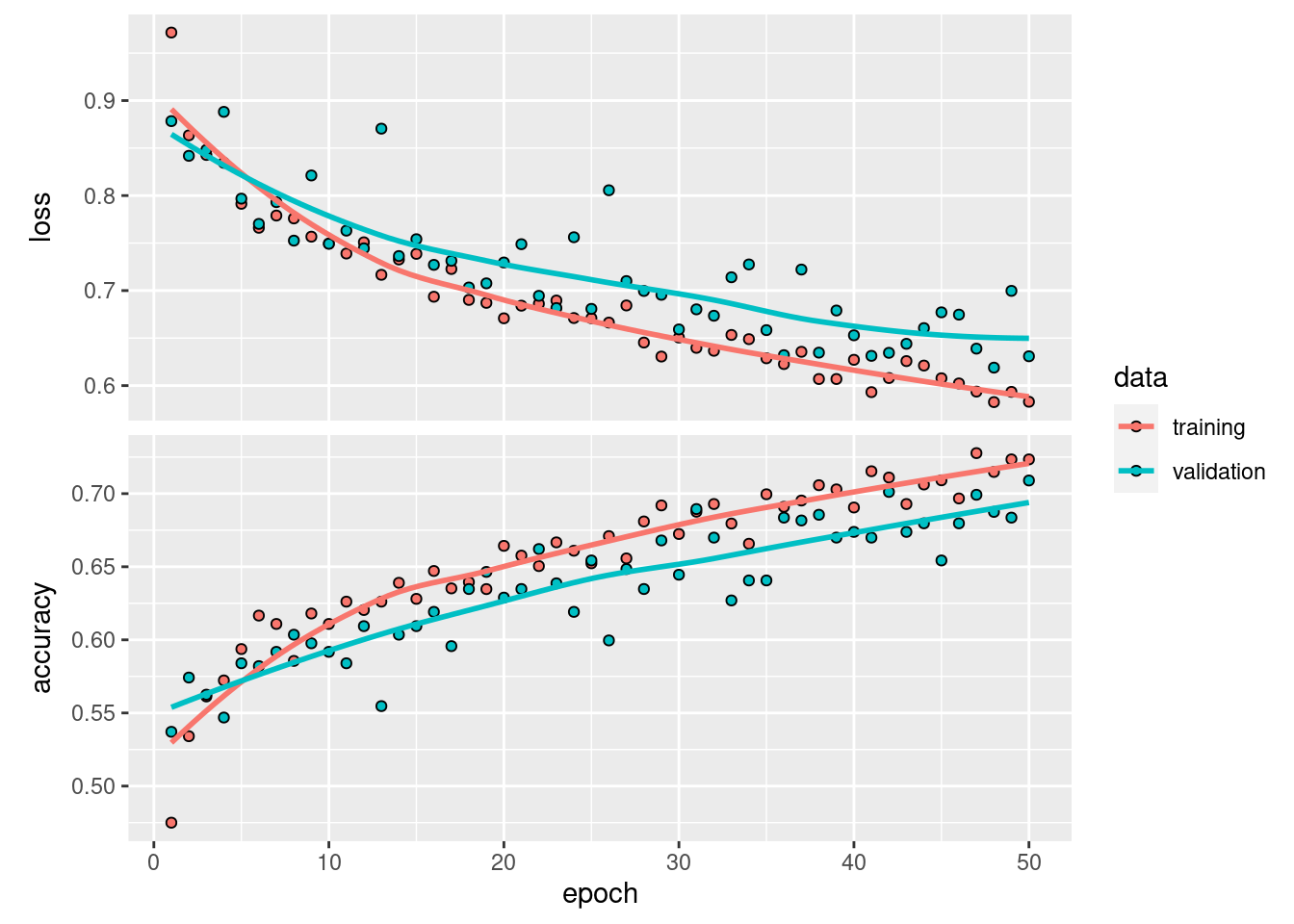
Model Evaluation
Now we will further evaluate the data and acquire the confusion matrix for the validation data.
pred_test <- predict_classes(model_big, test_x)

head(pred_test, 10)
#> [1] 1 0 0 1 0 2 0 0 0 0To get easier interpretation of the prediction, we will convert the encoding into proper class label.
# Convert encoding to label
decode <- function(x){
  case_when(x == 0 ~ "cat",
            x == 1 ~ "dog",
            x == 2 ~ "panda"
            )
}

pred_test <- sapply(pred_test, decode)

head(pred_test, 10)
#> [1] "dog" "cat" "cat" "dog" "cat" "panda" "cat" "cat" "cat"
#> [10] "cat"Finally, we evaluate the model using the confusion matrix. This model perform better than the previous model because we put more CNN layer to extract more features from the image.
confusionMatrix(as.factor(pred_test),
                as.factor(val_data$class)
                )
#> Confusion Matrix and Statistics
#>
#> Reference
#> Prediction cat dog panda
#> cat 122 54 5
#> dog 43 100 8
#> panda 12 24 162
#>
#> Overall Statistics
#>
#> Accuracy : 0.7245
#> 95% CI : (0.6844, 0.7622)
#> No Information Rate : 0.3358
#> P-Value [Acc > NIR] : < 0.00000000000000022
#>
#> Kappa : 0.5869
#>
#> Mcnemar's Test P-Value : 0.006952
#>
#> Statistics by Class:
#>
#> Class: cat Class: dog Class: panda
#> Sensitivity 0.6893 0.5618 0.9257
#> Specificity 0.8329 0.8551 0.8986
#> Pos Pred Value 0.6740 0.6623 0.8182
#> Neg Pred Value 0.8424 0.7942 0.9608
#> Prevalence 0.3340 0.3358 0.3302
#> Detection Rate 0.2302 0.1887 0.3057
#> Detection Prevalence 0.3415 0.2849 0.3736
#> Balanced Accuracy 0.7611 0.7085 0.9122Predict Data in Testing Dataset
After we have trained the model and if you have satisfied with the model performance on the validation dataset, we will do another model evaluation using the testing dataset. The testing data is located on the test folder.
df_test  <- read.csv("data_input/image_class/metadata_test.csv")

head(df_test, 10)
#> class file_name
#> 1 cat data_input/image_class/test/img_01.jpg
#> 2 cat data_input/image_class/test/img_02.jpg
#> 3 cat data_input/image_class/test/img_03.jpg
#> 4 cat data_input/image_class/test/img_04.jpg
#> 5 cat data_input/image_class/test/img_05.jpg
#> 6 cat data_input/image_class/test/img_06.jpg
#> 7 cat data_input/image_class/test/img_07.jpg
#> 8 cat data_input/image_class/test/img_08.jpg
#> 9 cat data_input/image_class/test/img_09.jpg
#> 10 cat data_input/image_class/test/img_10.jpgThen, we convert the image into 2D array.
test_x <- image_prep(df_test$file_name)

# Check dimension of testing data set
dim(test_x)
#> [1] 340 64 64 3The testing data consists of 341 images with dimension of 64 x 64 pixels and 3 color channels (RGB). After we have prepared the data test, we now can proceed to predict the label of each image using our CNN model.
pred_test <- predict_classes(model_big, test_x)

head(pred_test, 10)
#> [1] 0 0 0 0 0 0 0 0 0 1To get easier interpretation of the prediction, we will convert the encoding into proper class label.
# Convert encoding to label
decode <- function(x){
  case_when(x == 0 ~ "cat",
            x == 1 ~ "dog",
            x == 2 ~ "panda"
            )
}

pred_test <- sapply(pred_test, decode)

head(pred_test, 10)
#> [1] "cat" "cat" "cat" "cat" "cat" "cat" "cat" "cat" "cat" "dog"Finally, we evaluate the model using the confusion matrix.
confusionMatrix(as.factor(pred_test),
                as.factor(df_test$class)
                )
#> Confusion Matrix and Statistics
#>
#> Reference
#> Prediction cat dog panda
#> cat 88 44 1
#> dog 22 58 6
#> panda 1 4 116
#>
#> Overall Statistics
#>
#> Accuracy : 0.7706
#> 95% CI : (0.7222, 0.8142)
#> No Information Rate : 0.3618
#> P-Value [Acc > NIR] : < 0.0000000000000002
#>
#> Kappa : 0.6549
#>
#> Mcnemar's Test P-Value : 0.05186
#>
#> Statistics by Class:
#>
#> Class: cat Class: dog Class: panda
#> Sensitivity 0.7928 0.5472 0.9431
#> Specificity 0.8035 0.8803 0.9770
#> Pos Pred Value 0.6617 0.6744 0.9587
#> Neg Pred Value 0.8889 0.8110 0.9680
#> Prevalence 0.3265 0.3118 0.3618
#> Detection Rate 0.2588 0.1706 0.3412
#> Detection Prevalence 0.3912 0.2529 0.3559
#> Balanced Accuracy 0.7981 0.7138 0.9600Conclusion
Many data comes in different forms and not only in structured format. Some data may come in form of text, image, or even video. That’s where the conventional machine learning model hit its limit and that’s where Deep Learning shines. Deep Learning can handle different unstructured data by simply adjusting the network architecture.
 More details
 More details
Share this post
Twitter
Facebook
LinkedIn